1 Introduction
The world economy has shown exponential growth since the Industrial Revolution, and people's living standards and social modernization level have been significantly improved. However, with the consumption of fossil energy, CO
emissions have increased dramatically, causing serious adverse effects on the global environment and climate
[1]. The international community has reached a number of agreements on climate change, but further control is still needed. As the world's second largest economy with the highest carbon emissions, China has an important role in controlling global climate change. Chinese President Xi Jinping announced China's carbon peaking and carbon neutrality vision in 2020, demonstrating the country's commitment to reducing emissions and carbon emissions.
In order to reduce carbon emissions, we need to focus on densely populated and industrialized regions. According to the 14th Five-Year Plan, China will implement major regional strategies, including accelerating the coordinated development of Beijing-Tianjin-Hebei (BTH) region, comprehensively driving the development of Yangtze River Economic Belt, actively promoting the construction of Guangdong-Hong Kong-Macao Great Bay Area (GBA for short), speeding up the integrated development of Yangtze River Delta (YRD), and strengthening the ecological conservation and high-quality development of the Yellow River Basin
[2]. These five regions are the "main battlefield" of China's economic and social development, and also the "key areas" for reducing carbon emissions. Since these major strategic regions are different in economic base, development path and strategic positioning, the effect of reducing carbon emissions also varies from region to region. Therefore, using CEI as the main measurement indicator of carbon emission reduction to study the spatial differences and temporal evolution of CEI in Chinese cities and major strategic regions is of great significance for promoting green transformation and coordinated development
[3].
There are obvious differences in the economic foundation, development path and strategic positioning of different regions in China, and in the course of development in recent years, remarkable achievements have been made in emission reduction and carbon reduction. Therefore, this study is based on data such as carbon emissions, economic development, and industrial structure at the city level, and uses carbon emission intensity as a reference to carry out index measurement activities, so that it can be ranked according to the carbon emission intensity of different regions in the country and observe the entire development process. By using the Dagum Gini coefficient to analyze the differences in carbon emissions within and between regions, and to conduct a comparative study on the carbon emission intensity of each region based on the kernel density. Through the Moran's I and LISA distribution test, the spatial correlation of carbon emissions in prefectures and cities was tested, and the Geoda software was used to describe its spatial agglomeration characteristics, and a visualization map was produced. All these will contribute to the ultimate realization of the green transformation and upgrading development goals of domestic and major strategic regions.
Based on the calculation of carbon emission intensity at the city level, and with the help of the LDMI factor decomposition model, a quantitative study of the carbon emission intensity of the country and key regions was carried out, and the impact of each influencing factor on carbon emission was analyzed from four aspects: Population size, economic development, industrial structure, and technological level. Intensity effect. Carry out a corresponding analysis of the research content that has not yet been studied in the domestic and foreign research fields, and decompose and explore the carbon emission factors of differentiated industries. The ultimate goal is to comprehensively summarize its development laws and core development characteristics.
At present, the literature on the factors affecting carbon emissions rarely focuses on cities and urban agglomerations because there are no statistical indicators of carbon emissions at the prefecture-level city level. This paper calculates the carbon emission data and energy consumption structure data of 262 prefecture-level cities across the country through the indicators in the CEADS database and the city statistical yearbook. Five urban agglomerations, BTH, GBA, YRD, Chengdu-Chongqing urban agglomeration, and Harbin-Changchun urban agglomeration were selected as the research objects, and regional carbon emission differences can be described from the scale of urban agglomerations or cities. The granularity is refined to the city level, which fills the gap in the continuous long-term carbon emission data at the city level. It provides a basis for China to propose carbon emission reduction measures from the city level and urban agglomeration level in the future.
2 Literature Review
2.1 Calculation of the Carbon Emissions
Wu, et al. used a data-driven method, analyzed the efficiency and amount of carbon emission of each industrial sector after processing multi-dimensional data by the improved IPCC EF method of calculating carbon emissions
[4]. CEI refers to the amount of CO
emissions per unit of GDP. It reflects the relationship between pollution and economic growth, and is an important evaluation indicator of sustainable economic development
[2, 3]. Since there is no authoritative official agency directly releasing CO
emission data in China, CEI research is conducted. Firstly, CO
emissions need to be calculated. At present, the main calculation method is the exponential decomposition method, which calculates the total CO
emissions of a region or industry by multiplying and accumulating the consumption of different types of fossil energy and carbon emission factors
[5, 6]. Some researchers have also used the input-output method
[7], or the method of production decomposition analysis based on nonparametric distance function and environmental technology
[8].
2.2 Spatial Differences and Dynamic Evolution of Carbon Emissions
By building the GWR model, Wang, Shi and Fang emphasized urbanization and industrial structure strength will lead to changes in carbon dioxide emissions. The paper also expressed the correlation characteristics reflected in China's space in different years. The survey results show that urbanization can lead to a gradual increase in carbon dioxide emissions in various provinces and cities, and energy intensity and industrial structure will be affected to a certain extent. to the state of development
[9]. Wang, et al. used data of 30 provinces in China from 2004–2019 for Carbon emissions from the power sector, to test the spatial differences of Carbon emissions from the power sector among all provinces. The results showed differences and the global Moran's I shows significant positive spatial autocorrelation
[10]. Using the data of inter-provincial carbon emissions in China from 1995 to 2007, Yue, et al. descriptively analyzed the regional differences in carbon emissions in the eastern, central and western regions as well as the whole country. It was found that regional carbon emissions and per capita emissions were ranked from the east, central, and west in descending order, but the CEI of the central and western regions was much higher than that of the eastern region; inter-provincial differences within a region contributed more to the overall difference, while inter-regional differences contributed less to it
[11]. Lin and Huang studied the spatial characteristics of regional carbon emissions in China using a spatial econometric model and found that China's CEI was higher in the west than in the east; per capita carbon emissions were higher in the east than in the west; the diffusion level of per capita carbon emissions was higher than that of CEI; and there was a strong spatial agglomeration effect for both CEI and per capita carbon emissions
[12]. Liu and Zhao used the Gini coefficient and its subgroup decomposition method proposed by Dagum to measure the national CO
emission Gini coefficient based on the CEI of three regions: East, West and Central. Their study showed that there were obvious regional differences in CO
emission intensity in China, and such regional differences showed a trend of increase but were not significant; the inter-regional difference in carbon emissions contributed more to the overall difference, the intra-regional difference did not contribute significantly, and the contribution of hyper-variable density also showed a trend of decrease
[13]. Liu, Bao and Yang measured the regional differences of agricultural carbon dioxide emissions in China by using the Dagum Gini coefficient decomposition method in combination with the non-parametric estimation method. Their study showed that the spatial differences in agricultural carbon emissions in China showed a general trend of narrowing, with inter-regional disparity being the main source of the overall disparity; the CEI of different levels of agriculture had poor intergroup mobility; and the overall agricultural carbon emissions showed an upward trend toward medium-high and high levels
[14].
2.3 Influencing Factors of Carbon Emissions
Ding, Zhang and Yang used a multidimensional decomposition approach which combines PDA and IDA. This approach illustrate how energy structure effect, efficiency change effect and technical change affect carbon emission intensity of China's 30 provinces. The research results show that output biased technical change is the critical factor in carbon emission intensity
[15]. Wu, et al. used the LMDI decomposition method for data modeling to measure the contribution of energy efficiency, industrial structure, GDP per capita, and population size to carbon emission changes, to identify targets for industrial carbon reduction, and to propose a targeted optimization path for carbon emission
[4]. Compared to the traditional way of capturing the drivers of carbon emissions, Liu, et al. generated a more general method of Divisia Index method to find the influencing factors. The results showed that investment activity is a primary factor in promoting China's carbon emissions, followed by energy use and economic activities
[16]. Fu, et al. introduced the concepts of spatial dependence and spatial variability and constructed a STIRPAT model to analyze the spatial dependence of provincial CEI in China. They found that factors such as population structure, energy intensity, energy structure, and industrial structure had significant effects on CEI
[17]. Zhou and Jiang used the dynamic spatial Durbin model to study the influencing factors of inter-provincial CEI in China from the perspective of effect decomposition, and concluded that economic growth and technological input had direct negative spatial effects on CEI, industrial structure, energy intensity and energy consumption structure had direct positive spatial effects on CEI, technological input had negative spatial spillover effects, and energy intensity had positive spatial spillover effects
[18]. City-level studies are neither as many as nor as deep as provincial-level studies. Wang, et al. were among the first to study the relationship between CEI and urban spatial layout of 35 major cities in China, but their research was more from the perspective of land utilization than from the perspective of economics
[19]. The existing literature about the research on carbon emission intensity has shown an increasing trend in recent years, there is still a lot of room for research in this field. First, in the measurement of carbon emissions, the current methods all rely on energy statistical data, which has brought about two potential problems: On the one hand, some local governments have limited control over carbon emissions due to performance appraisal. Energy data in bad years may not be disclosed or have false reports, which will affect the accuracy of the calculation results of carbon dioxide emissions. And there may even be large deviations in some areas. Second, most of the existing literatures focus on provinces, while there are few literatures on cities, and there are not many literatures on regional studies based on cities. Third, the exploration of the characteristics of carbon emission intensity mostly uses the spatial econometric model to carry out convergence research, while the quantitative analysis research on the regional differences and dynamic evolution of carbon emission intensity is relatively lacking. In view of this, this paper uses city-level data to carry out research on the regional differences, dynamic evolution and influencing factors analysis. First, based on the carbon emission data released by CEADs, the carbon emission intensity of 262 cities above the prefecture level in the country is calculated, which is the main research object of the paper. Secondly, the Dagum Gini coefficient and its decomposition method and The kernel density estimation method is used to study the regional differences and dynamic evolution characteristics of carbon emission intensity in major strategic regions across the country. Finally, an LDMI method is established to study the influencing factors of carbon emission intensity in cities and major strategic regions. National and regional emission and carbon reduction policies have been introduced in major strategic regions to accelerate the pace of carbon peaking and carbon neutralization to provide quantitative support.
3 Methodology and Data
3.1 Dagum Gini Coefficient and Its Decomposition
In this paper, the Dagum Gini coefficient and the overall difference of the sample is decomposed into three parts: Intra-group difference, inter-group net difference and inter-group hyper-variable density to measure the spatial difference of CEI in China
[20]. Dagum Gini coefficient is defined as follows:
wherein, and are the serial numbers of two specific regions, and represent the number of cities in the corresponding regions, and denote the CEI of the city in the region and that of the city in the region, respectively, and and represent the average value of CEI of all cities in the corresponding regions.
The Dagum Gini coefficient is further decomposed into the following three parts
[20]:
wherein, represents the ratio of the number of cities in the region to the sample size , and represents the ratio of CEI in the region to the CEI of all cities in the sample. From , it can be known that the overall Dagum Gini coefficient is the weighted average of the inter-group (intra-group) Gini coefficient of all pairwise combinations in all regions, and the corresponding weight is . stands for the total contribution of urban CEI differences in each region to the overall difference, stands for the total contribution of all regional differences, and stands for the relative influence between region and region.
Therefore, if the CEI of the regions with higher average CEI is reduced and the CEI of the regions with lower average CEI is increased, then the overall Gini coefficient can be reduced by narrowing inter-regional differences. But in fact, if there is overlapping between sub-samples, that is, the CEI of some high-carbon cities in low-carbon regions is greater than the CEI of some low-carbon cities in high-carbon regions, then, raising the CEI of the former while lowering that of the latter may increase the Gini coefficient within regions, reduce the net difference between regions, aggravate the inequality of overlapping parts between regions, and make the overall Gini coefficient rise rather than fall. This part of Gini coefficient caused by an overlap between groups is called inter-group hyper-variable density. If there is no overlap between groups, its value is 0.
3.2 Kernel Density Estimation (KDE)
KDE is an important nonparametric estimation method, which can be intuitively understood as a "smoothened" histogram, and can describe the distribution characteristics of urban CEI with a continuous density curve
[21]. The horizontal position of the kernel density curve of single-period sample data in can represent the level of CEI, the height and width of the curve peaks can reflect the concentration degree of CEI in the period, the number of peaks can describe the polarization degree of the sample data, and the distribution ductility, i.e., the degree of curve tailing, can describe the distance from the city with the highest or lowest CEI to other cities. The longer the curve tail, the bigger the intra-regional difference. The dynamic evolution of CEI distribution characteristics in the same region can be identified by vertically comparing the kernel density curves of multi-period samples in the same region, and the differences in CEI variation trajectories can be captured by horizontally comparing the shapes of kernel density curves in multiple regions
[21]. The kernel density curve of CEI in the
region is generated by the following function:
wherein, represents the kernel density function, which describes the weight of all sample points in the neighborhood, and represents the window width of KDE. Commonly used kernel density functions are Gaussian, Epanechnikov, bipartite and triangular kernel density functions, but in general, choosing different kernel density functions has little effect on the estimation results, so this paper uses the most common Gaussian kernel function. The paper chooses the optimal window width produced by the system. The smaller the window width, the more accurate the estimate, but the number of samples included in the calculation in the interval will also decrease accordingly, resulting in a large variance of estimate and poor smoothness of the density curve.
3.3 LDMI Decomposition Model
In this paper, population size, economic development level, industrial structure and technological progress are selected as the influencing factors of carbon emissions, and the carbon emissions, population size, and GDP of the cities in each UA and the carbon emissions and GDP of different industries are selected to carry out an empirical study on complete decomposition of carbon emissions in five different regions
[22]. Due to the requirements of LMDI method for carbon emission data of different industries, it is difficult to make a complete factor decomposition calculation of carbon emissions including industrial structure changes at the scale of prefecture-level cities. Therefore, this paper modifies the traditional LMDI method to fill in the gap in the research of carbon emission factor decomposition with industrial information at the current scale of prefecture-level cities, in an attempt to reveal the more universal characteristics and laws of carbon emission.
The specific calculation method is shown below. Assuming that the carbon emission of the
region is
, then the emission can be decomposed according to Formula (5)
[23]:
wherein, is the population size of the region, is the GDP of the ith region, is the added value of the industry in the region, and is the carbon emission of the industry in the region.
For simplicity, let
, and
, where
is GDP per capita, representing the level of regional economic development,
is the share of the added value of regional industries in regional GDP, and
is the CEI of the regional tertiary industry, representing the technology level of the tertiary industry
[24].
wherein, is:
The modified LMDI decomposition method in this paper has the following advantages. Firstly, it can completely decompose the temporal variation of regional carbon emissions, and there is no residual value. Secondly, at the industry level, the calculation method of observing the contribution of industrial structure changes makes the relationship between complex economic structure characteristics and carbon emissions into a concise quantitative relationship, which is easy to understand and compare. The method of calculating the contribution of regional technology level changes is similar. Therefore, the decomposition calculation formula of regional carbon emission change based on the LMDI method can not only achieve no residual value in calculation, but also make complex economic phenomena more concise, more objectively interpretable in economics
[25].
3.4 Research Data
To calculate the regional CEI, we need to know the regional CO
emissions and regional GDP. Regional CO
emissions are the sum of carbon emissions of all cities in the region. Referring to the practice of Wu and Guo
[26], this paper calculates the carbon emissions from the consumption of electricity, gas, liquefied petroleum gas and heat energy in 262 sample prefecture-level cities by using the set carbon conversion factor and carbon emission coefficient
[2, 4].
The urban carbon emission data, urban GDP and urban population data required for calculation mainly come from Urban Statistical Yearbook of China, China Statistical Yearbook, Urban Construction Statistical Yearbook of China, and China Regional Statistical Yearbook. The data of regional GDP were collected from Urban Statistical Yearbook of China, using the city-wide statistical caliber.
The research object of this paper is China's five national strategic regions: The northeast region, southeast coastal region, north region, south region and the west region. The five regions are in different and representative development stages. After a comprehensive evaluation of data quality, the sample time span selected in this paper is from 2006 to 2019.
Using the method described above, the authors calculated the CEI of 262 cities and 5 UAs across China. The average annual CEIs from 2006 to 2019 are shown in Figure 1.
Figure 1 Changes of regional average CEI |
Full size|PPT slide
On the whole, the average CEI nationwide has gradually decreased from 7.35 kilotons/100 million yuan in 2006 to 3.611 kilotons/100 million yuan in 2019, with an average annual decrease of 5.62%, which shows that China had made great progress in reducing carbon dioxide emissions and great contributions to the global efforts to deal with climate change. By region, the CEI of the YRD region was 5.55 kilotons/100 million yuan in 2006, the lowest among all regions, followed by that of the Chengdu-Chongqing urban agglomeration (CCUA), 6.29 kilotons/100 million yuan. In 2012, the CEI of CCUA dropped to 3.24 kilotons/100 million yuan, lower than that of YRDUA, and the average CEI of the two regions was lower than the national average of 4.65 kilotons/100 million yuan for a long time. Since the 18th CPC National Congress, the carbon emissions of CCUA have been on the decline, which is the result of the continuous improvement of regional industrial structure and the gradual transformation of energy structure from conventional to clean, low-carbon energies. The five regions of BTH, YRD, GBA, CCUA and the Harbin-Changchun urban agglomeration (HCUA) show a spatial pattern of "low in the south but high in the north" on the whole, which is consistent with the basic situation of "strong in the south and weak in the north" in China's urban development.
3.5 Theoretical Basis
Due to the influence of geographical environment, location conditions, policy measures, etc., there are huge differences in economic and social development between regions. Therefore, when allocating carbon emission reduction responsibilities, it is very important to grasp the characteristics of temporal and spatial differentiation between regions. Existing research assumes that each region is spatially independent, builds a classic linear regression model based on time series data, divides all regions of the country into different carbon emission levels and different regional categories, and explores carbon emissions through methods such as Gini coefficient and Theil index. The differences of various indicators and influencing factors between regions and within regions
[27].
However, China's regional differences are huge, and geographical factors vary greatly, so carbon emissions and influencing factors in different regions will be different. Therefore, the research on carbon emission regions under the global regression model ignores the spatial non-stationarity of each region and covers up the connection and agglomeration of each region in space
[28].
By using China's inter-provincial carbon emission data from 1995 to 2007, the regional differences in carbon emissions in the eastern, central, and western regions of China are studied. Through research, we know that the order of China's regional carbon emissions and per capita emissions from high to low is the east, central and west, but the fact is that the carbon emissions in the central and western regions are very high, far exceeding those in the eastern regions; The contribution of inter-provincial differences and inter-regional differences to China's inter-provincial carbon intensity differences is relatively large and the other is relatively small
[8].
Aiming at the spatial characteristics of China's regional carbon emissions, through the construction of a spatial econometric model, we learned that China's carbon emissions are clearly high in the west and low in the east, and the per capita carbon emissions have become high in the east and low in the west. The diffusion of carbon emission intensity is relatively high, but whether it is per capita carbon emission or carbon emission intensity, both have a strong aggregation effect
[29].
Through the Gini coefficient and subgroup decomposition method developed by Dagum, the Gini coefficient of carbon emissions is calculated based on the intensity of carbon emissions in the three major regions of the east, west, and central regions. Through the analysis, it is concluded that China's carbon dioxide emission intensity is not balanced among regions, and this imbalance is still increasing, and the increase in knowledge is not obvious; the differences in carbon emissions in various regions and the contribution of intra-regional differences are different. The former increases significantly while the latter increases only slightly, and the contribution rate of hypervariable density also shows a downward trend
[30]. Taking per capita carbon emissions and carbon emissions as research indicators, and combining these two indicators with the measurement function of Theil index, the three regions and eight regions were calculated, and the regional differences between the two were obtained. Through the calculation results, it can be known that regional differences in China. It is very obvious, and the regional differences in carbon emission intensity are significantly higher than the regional differences in per capita carbon emissions; the measurement results of the differences in the three regions and the regions come from the inside and outside of the region respectively
[27].
Combining the Dagum Gini coefficient decomposition method with the non-parametric estimation method, the regional differences of China's carbon dioxide emissions are calculated. From the calculation results, it can be known that the differences between regions in China's carbon emissions are getting smaller and smaller, and the main gaps come from between regions; the inter-group mobility of the differences in carbon emission intensity is not good. According to the data, carbon emissions will rise again and gradually develop towards high emissions
[31].
Some researchers also realize that the final research conclusions will be affected to a certain extent due to different regional characteristics and inconsistent levels of economic development. Therefore, the research object is divided according to the region, and the research work is carried out in a targeted manner. By selecting more than 20 cities in China as research samples, it is emphasized that if China is divided into three regions, the scale of carbon emissions will increase significantly as the rate of urbanization increases, but the driving force is not significant
[32]. Collected data samples from 30 provinces across the country, with a time span from 1998 to 2010, went abroad to analyze the data and found that the urbanization process in the eastern and central regions of China did not affect carbon emissions, while the cities and towns in the western region The pace of globalization has a significant impact on carbon emissions
[33]. Using the upgraded panel data for analysis, it is finally concluded that urbanization has played a role in promoting carbon emissions in the eastern region. Through the analysis of technical factors, population size, and urbanization indicators, it is found that urbanization has an impact on carbon emissions. The relationship between urbanization and carbon emissions in the central region is an inverted U-shaped; urbanization in the western region does not have a driving effect on carbon emissions, but has a negative effect
[34].
The dynamic panel was used for analysis, and it was concluded that the urbanization level of the central and western regions would reduce carbon emissions, while the eastern region had a positive proportional relationship between the two
[35]. Based on the analysis of provincial panel data in a fixed period in China, it finally shows that the urbanization development in the eastern region of China can form a strong driving effect; on the basis of urbanization changes, the central and western regions will gradually enter a state of carbon peaking, and then urbanization. The higher the level of development, the lower the carbon emissions, and there is an obvious inverted U-shaped relationship between urbanization and carbon emissions. A large part of the sample cities in the central and western provinces have a relatively high level of urbanization development, and have even exceeded the U-shaped inflection point.
Therefore, even if the urbanization process continues to deepen, carbon emissions will not increase
[36]. Using the panel data between 2000 and 2010 as the research basis, the research samples were selected nationwide. The results of the survey prove that the impact of urbanization level on carbon emissions has obvious positive driving characteristics. Moreover, the current relationship between urbanization development and carbon emissions is not dominated by an inverted U-shaped relationship, and the Kuznets curve has not yet formed. Therefore, as the level of urbanization increases, economic development will not continue to be a key factor affecting carbon emissions.
Secondly, it is distinguished according to geographical location, mainly including the eastern and non-eastern regions. The research results prove that the impact of urbanization on carbon emissions in any region is still mainly positive, but the impact of this type of driving effect in non-eastern regions is far greater than that in eastern regions
[37]. After the construction of different development models, mathematical expressions are finally used for effective derivation, so that the degree of industrial structure adjustment will also change. After the level of urbanization development enters a higher level, the per capita carbon emissions will also be significantly suppressed
[38].
Referring to the results of theoretical analysis, empirical analysis and testing are carried out on panel data, and it is finally emphasized that there is no linear relationship between the level of urbanization development and carbon emissions, but the Kuznets inverted U-shaped relationship already exists. Then, the inflection point time of per capita carbon emissions in different provinces and cities is calculated, from which we can learn that, except for Liaoning and other provinces in the eastern region, the per capita carbon emissions of other provinces and regions have exceeded the inflection point time. However, if the provinces in the central and western regions want to achieve this target, it may take about 15 years. Taking 30 provinces and cities as the research object, it comprehensively expounds the time impact that urbanization and economic development can have on carbon emissions. Finally, the research results prove that the urbanization development in the central and eastern regions can form a strong driving force for both carbon emissions and per capita carbon emissions, and the carbon Kuznets curve has been confirmed to exist. On the contrary, the western region has little impact on carbon emissions, and economic development has not created a carbon Kuznets curve, which is mainly based on a positive linear development relationship
[39]. In the whole country, as well as in the eastern region, the relationship between urbanization development and carbon emissions is the same, that is, the inverted N-type relationship. This is not the case in the central and western regions, where the N-type relationship is dominant, and the impact effect is not obvious
[38].
4 Spatial Differences and Dynamic Evolution of Regional CEI
4.1 Nationwide and Intra-Regional Differences in Carbon Emissions
Using Dagum Gini coefficient, the author calculated the intra-group differences of CEI in 262 cities and 5 UAs in China. The calculation results for the sample period of 2006–2019 are shown in Figure 2.
Figure 2 Changes of intra-group differences of regional CEI |
Full size|PPT slide
From a national perspective, the overall Gini coefficient of China's CEI was quite high, with an average value of 0.28 in the sample period. Except for a slight decline in the years of 2008–2013, it maintained a growth trend in other years, indicating that China's urban CEI was increasingly uneven. From a regional perspective, from 2006 to 2014, the intra-group Gini coefficient of the YRD region exceeded the national Gini coefficient, indicating that internal imbalance in the YRD region was serious, while the Gini coefficient of other UAs in the sample period did not exceed the national level, suggesting that the degree of imbalance was low, and the overall difference was mainly due to inter-regional differences. The Gini coefficient of the HCUA region was low in 2006, and only 0.13 in 2010, but it maintained rapid growth after 2010, reaching a peak of 0.28 in 2016, which suggests that the high-quality development in HCUA was obviously unbalanced and insufficient, and the paces of industrial transformation, energy conservation and emission reduction were inconsistent. The average Gini coefficient of the GBA region was only 0.18, which was consistent with the fact that the industrial division of labor within GBA was clear and the division of labor between upstream and downstream industries was basically clear.
4.2 Inter-Regional CEI Differences
The inter-group Gini coefficient proposed by Dagum
[20] is used to measure inter-regional CEI differences, with results shown in
Table 1.
Table 1 Inter-regional CEI differences |
| | BTH-GBA | BTH-YRD | BTH-HCUA | BTH-CCUA | GBA-YRD | GBA-HCUA | GBA-CCUA | YRD-HCUA | YRD-CCUA | HCUA-CCUA |
| 2006 | 0.2591 | 0.3480 | 0.2833 | 0.2808 | 0.3216 | 0.2512 | 0.2428 | 0.3895 | 0.3011 | 0.3133 |
| 2007 | 0.2648 | 0.3529 | 0.2725 | 0.3123 | 0.3146 | 0.2105 | 0.2650 | 0.3568 | 0.3159 | 0.2959 |
| 2008 | 0.2598 | 0.3456 | 0.2688 | 0.3009 | 0.3258 | 0.2090 | 0.2688 | 0.3560 | 0.3078 | 0.2959 |
| 2009 | 0.2531 | 0.3498 | 0.2421 | 0.3059 | 0.3251 | 0.1746 | 0.2690 | 0.3147 | 0.3072 | 0.2538 |
| 2010 | 0.2406 | 0.3294 | 0.2272 | 0.3003 | 0.3117 | 0.1727 | 0.2752 | 0.3068 | 0.3020 | 0.2694 |
| 2011 | 0.2312 | 0.2921 | 0.2184 | 0.2755 | 0.2775 | 0.1782 | 0.2582 | 0.2587 | 0.2757 | 0.2364 |
| 2012 | 0.2341 | 0.2768 | 0.2099 | 0.2564 | 0.2774 | 0.1856 | 0.2627 | 0.2438 | 0.2504 | 0.2270 |
| 2013 | 0.2216 | 0.2652 | 0.2110 | 0.2657 | 0.2474 | 0.1861 | 0.2480 | 0.2313 | 0.2465 | 0.2294 |
| 2014 | 0.2174 | 0.2646 | 0.2004 | 0.3107 | 0.2709 | 0.1982 | 0.3162 | 0.2482 | 0.2673 | 0.2912 |
| 2015 | 0.2191 | 0.2903 | 0.2598 | 0.3352 | 0.2633 | 0.2313 | 0.3143 | 0.3342 | 0.2636 | 0.3982 |
| 2016 | 0.1922 | 0.2780 | 0.2784 | 0.3290 | 0.2509 | 0.2586 | 0.3075 | 0.3696 | 0.2543 | 0.4380 |
| 2017 | 0.1844 | 0.2925 | 0.2524 | 0.3504 | 0.2520 | 0.2431 | 0.3037 | 0.3587 | 0.2589 | 0.4244 |
| 2018 | 0.1885 | 0.3240 | 0.2325 | 0.3856 | 0.2647 | 0.2339 | 0.3096 | 0.3644 | 0.2563 | 0.4257 |
| 2019 | 0.1913 | 0.3285 | 0.2212 | 0.3871 | 0.2659 | 0.2086 | 0.3130 | 0.3485 | 0.2504 | 0.4063 |
On the whole, the polygon's area in Figure 3 first expanded and then decreased, indicating that the trend of regional CEI divergence in China gradually expanded at first. Then, some regions reduced CEI by upgrading their industrial structure and applying high-tech technologies, so the area of the polygon gradually decreased after 2015.
Figure 3 Variations of inter-group CEI differences in the five regions |
Full size|PPT slide
4.3 Overall Difference and Decomposition of CEI
Using the above method, the overall difference of sample data can be decomposed into three parts: Intra-group contribution, inter-group net contribution and inter-group hyper-variable density. The absolute values and relative shares of each part are reported as follows.
The intra-group Gini coefficient of CEI in the five regions was 0.065 in 2006 and began to decline after 2010, falling to 0.05 in 2019. However, because inter-group differences rose faster in the sample period, the contribution rate of intra-group differences decreased from 20.96% in 2006 to 17.84% in 2019, while the overall contribution rate of inter-regional differences increased from 38.82% to 58.75%, which are the main source of overall regional CEI differences in China.
The value of inter-group net difference was 0.12 in 2006, decreased to 0.07 in 2013, and then began to increase, reaching 0.17 in 2019. It can be seen that the inter-group net difference showed an obvious "U"-shaped change. Its contribution rate to the overall regional difference decreased from 38.22% in 2006 to 29.74% in 2013, and then continuously rose to 58.75%.
During the sample period, both the net value and the contribution rate of inter-group hyper-variable density showed a steady increase at first and then decreased. The former was 0.12 in 2006, gradually increased to 0.14 in 2009, and then declined to 0.066 in 2019, while the latter gradually increased from 40.22% in 2006 to 47.64% and then decreased to 23.41%. Inter-group hyper-variable density reflects the contribution of the overlapping parts of sub-samples to the overall difference, and its share in the research results of this paper is small, which means that the division of five strategic regions can effectively distinguish between different types of cities and has strong rationality.
Figure 4 Spatial differences of CEI and their sources |
Full size|PPT slide
4.4 Dynamic Evolution of Regional CEI
The research based on Dagum Gini coefficient reveals the numerical level and specific sources of the overall differences of China's urban CEI, and identifies the change trajectory of relative differences among regions, but it cannot describe the temporal evolution process of the absolute CEI differences among regions. Therefore, this paper uses the KDE method to describe the distribution characteristics of sample data of each region, focusing on key attributes such as the distribution location of the corresponding density curve, the distribution form of the main peak, the distribution ductility and the number of peaks.
Starting from 2006, the kernel density curve of nationwide CEI showed a trend of overall shift to the left, indicating that the CEI in most cities was on a downward track, and the concepts of energy conservation, emission reduction, low-carbon development and sustainable development penetrated into local governments, and emission reduction achieved phased results. The distribution curves of the five regions in this study showed different trends, among which the curves of YRD and CCUA moved to the left, while those of the other three UAs moved to the right, which meant that BTH, GBA and HCUA were under great pressure to reduce carbon, so it was urgent to implement a series of industrial upgrading policies and issue a series of environmental policies in these three regions.
Table 2 Characteristics of the dynamic evolution of regional CEI |
| Name of region | Distribution location | Distribution form of main peak | Distribution form | Number of peaks |
| Nationwide | Left shift | Height decreases;
width increases | Right tailing | Single peak |
| BTH | Right shift | Height increases;
width decreases | Right tailing | Single or double peak |
| GBA | Right shift | Height increases;
width decreases | Right tailing | Single or double peak |
| YRD | Left shift | Height increases;
width decreases | Right tailing | Single peak |
| HCUA | Right shift | Height first rises and then falls; width increases | Left tailing | Double peak |
| CCUA | Left shift | Height increases;
width does not change | Right tailing | Double peak |
Figure 5 Dynamic evolution of regional CEI |
Full size|PPT slide
The national kernel density curve shows that the height of the main peak decreases and the width increases, which means that the dispersion degree of urban CEI in the sample is on the rise. Due to the different industrial bases in different regions, the path selection and difficulty of carbon emission reduction are quite different. The heights of the main peaks of the distribution curves of BTH, GBA and YRD increase and the width decrease, which shows that the absolute CEI difference among cities in these region is gradually narrowing.
Both the national distribution curve and the distribution curves of BTH, GBA, YRD and CCUA show significant right tailing, indicating that the CEI of some cities is significantly higher than that of other cities in the same region. Some left trailing exits in the distribution curve of HCUA, which means that the carbon emissions of core cities such as Harbin and Jilin are much lower than those of other cities in the same region.
Two peaks exist in the distribution curves of the country and the five regions during the sample period, which shows that the CEI of cities in the same region is polarized. The distance between the main peak and the side peak of HCUA and CCUA is large, indicating that there is spatial polarization in these two regions. In 2019, the double-peak phenomenon in each region gradually weakened and the curves became single-peaked, suggesting that the degree of differentiation within the same region gradually decreased.
5 Analysis of Influencing Factors of Regional Carbon Emissions
As mentioned afore, the research sample covers 262 cities and five regions: BTH, YRD, GBA, HCUA and CCUA; the sample period is 2006–2019. The carbon emission data of each region are the carbon emissions generated by the consumption of electricity, gas, liquefied petroleum gas, and heat. For the data of added value by industry, the primary industry includes agriculture, forestry, animal husbandry and fishery, the secondary industry includes manufacturing, construction, mining and so on, and the tertiary industry includes transportation, communication, sales, catering, household consumption, etc.
In this paper, population size, economic development level, industrial structure and technological progress are selected as the influencing factors of carbon emissions, and based on the population size, carbon emissions, GDP, and industry-specific GDP of each prefecture-level city in the UAs, an empirical study is carried out on the complete decomposition of carbon emissions in the five different regions.
5.1 Contribution and Intensity of Various Influencing Factors of Carbon Emissions
Based on the modified LMDI method, it was found that nationwide carbon emissions increased year on year from 2007 to 2019, that is, . The contribution of each influencing factor and its share in the total effect on carbon emissions provide more detailed information.
Table 3 Carbon emissions and related data in BTH region from 2006 to 2019 |
| | CO2 emissions (10, 000t) | GDP (10, 000yuan) | CEI (kiloton of CO2/100 million yuan) | Population size (10, 000) | Population industry GDP (10, 000 yuan) | Secondary industry GDP (10, 000 yuan) | Tertiary industry GDP (10, 000 yuan) | Scientific and technological R&D expenditure (10, 000 yuan) | Urbanization rate (%) | Employees (10, 000) | Labor productivity |
| 2006 | 20825.32 | 236870595.00 | 98.22 | 9091.36 | 17852859.17 | 100344825.56 | 118672810.27 | 248285.00 | 45.26 | 1208.51 | 22.18 |
| 2007 | 24512.76 | 283092308.00 | 95.71 | 9211.94 | 19773830.35 | 116979283.52 | 146340194.13 | 1261908.00 | 46.59 | 1241.99 | 25.88 |
| 2008 | 25272.92 | 336010330.00 | 78.39 | 9344.41 | 22640509.97 | 139964884.92 | 173404454.22 | 1570687.00 | 48.05 | 1271.09 | 30.75 |
| 2009 | 26487.68 | 361918859.00 | 76.72 | 9448.76 | 23906000.91 | 146414311.79 | 191599176.30 | 1801699.00 | 50.78 | 1324.07 | 32.15 |
| 2010 | 28156.08 | 424108488.00 | 69.06 | 9541.05 | 28306856.76 | 172289009.49 | 223511921.75 | 2438281.00 | 50.08 | 1371.86 | 36.55 |
| 2011 | 27940.27 | 499128694.00 | 57.97 | 9619.12 | 32197721.71 | 205225619.64 | 261703592.44 | 2691179.00 | 51.26 | 1509.57 | 40.08 |
| 2012 | 29580.08 | 548794117.00 | 55.79 | 9707.22 | 35297936.90 | 222231540.22 | 291261615.59 | 3120856.00 | 52.40 | 1626.86 | 39.79 |
| 2013 | 31885.97 | 594194598.00 | 57.51 | 9744.86 | 37184109.15 | 233266650.51 | 323742082.27 | 3645908.00 | 53.70 | 1689.52 | 40.56 |
| 2014 | 33362.91 | 630743417.00 | 57.95 | 9942.96 | 37954889.70 | 238676686.23 | 354104413.98 | 4304588.00 | 54.78 | 1711.97 | 42.17 |
| 2015 | 32990.13 | 664001800.00 | 54.57 | 10021.91 | 38294900.00 | 235880300.00 | 389826600.00 | 4423363.00 | 56.52 | 1710.77 | 44.94 |
| 2016 | 32779.71 | 715160418.00 | 51.81 | 9920.88 | 39091032.88 | 247050136.98 | 429021248.14 | 4636697.00 | 58.30 | 1712.24 | 48.85 |
| 2017 | 33036.07 | 764010800.00 | 52.49 | 9904.55 | 33652500.00 | 254848800.00 | 475509500.00 | 5285306.00 | 59.72 | 1669.69 | 56.17 |
| 2018 | 35028.56 | 806341713.00 | 54.24 | 10001.22 | 35715022.20 | 245509630.57 | 525111977.62 | 5892235.00 | 60.98 | 1629.64 | 59.26 |
| 2019 | 35876.01 | 845017592.65 | 55.10 | 10081.10 | 38195277.00 | 242039774.64 | 564782541.00 | 6061436.00 | 62.13 | 1628.96 | 59.57 |
Contribution of population size: The contribution of population size is always positive, and it decreases slightly, indicating that it has a stable positive effect on the growth of carbon emissions. The larger the population, the less its share in the total effect on carbon emission change.
Contribution of economic development: The contribution of economic development level is positive, and is obviously bigger than that of population size. In other words, economic development has a greater impact on the increase of carbon emissions than population growth. The research shows that carbon emissions are still rising in the process of economic development during the sample period, having not reached the peak yet.
Table 4 Decomposition of the contribution of various influencing factors to the change of national carbon emissions from 2007 to 2019 |
| Year | Total effect | Population size | | Economic development level | | Industrial structure | | Technology level |
| Contribution | Share (%) | Contribution | Share (%) | Contribution | Share (%) | Contribution | Share (%) |
| 2007 | 0.0857 | 0.0052 | 0.0603 | | 0.2025 | 2.3634 | | 0.0092 | 0.1077 | | 0.1128 | 1.3160 |
| 2008 | 0.0323 | 0.0051 | 0.1574 | 0.1621 | 5.0230 | 0.0015 | 0.0456 | 0.1364 | 4.2260 |
| 2009 | 0.0813 | 0.0049 | 0.0599 | 0.0829 | 1.0192 | 0.0149 | 0.1828 | 0.0084 | 0.1038 |
| 2010 | 0.0750 | 0.0048 | 0.0639 | 0.1628 | 2.1723 | 0.0092 | 0.1221 | 0.1018 | 1.3583 |
| 2011 | 0.1007 | 0.0061 | 0.0609 | 0.1627 | 1.6168 | 0.0008 | 0.0075 | 0.0690 | 0.6853 |
| 2012 | 0.0380 | 0.0074 | 0.1953 | 0.0913 | 2.4002 | 0.0177 | 0.4645 | 0.0430 | 1.1309 |
| 2013 | 0.0488 | 0.0059 | 0.1210 | 0.0903 | 1.8521 | 0.0203 | 0.4160 | 0.0272 | 0.5570 |
| 2014 | 0.0087 | 0.0067 | 0.7674 | 0.0752 | 8.6031 | 0.0180 | 2.0603 | 0.0726 | 8.3100 |
| 2015 | 0.0211 | 0.0049 | 0.2330 | 0.0631 | 2.9830 | 0.0387 | 1.8315 | 0.0504 | 2.3842 |
| 2016 | 0.0003 | 0.0065 | 21.9319 | 0.0737 | 247.5626 | 0.0223 | 74.8595 | 0.0576 | 193.6333 |
| 2017 | 0.0163 | 0.0056 | 0.3428 | 0.1030 | 6.3315 | 0.0058 | 0.3574 | 0.0982 | 6.0317 |
| 2018 | 0.0224 | 0.0038 | 0.1688 | 0.0959 | 4.2857 | 0.0024 | 0.1092 | 0.0749 | 3.3452 |
| 2019 | 0.0179 | 0.0033 | 0.1855 | 0.0673 | 3.7608 | 0.0210 | 1.1733 | 0.0317 | 1.7728 |
| Note: In this table, "share" refers to the percentage of contribution of changes in various influencing factors in the total effect of changes in carbon emissions in a year. |
Contribution of industrial structure: The contribution of industrial structure is mostly negative. It can be seen that the optimization and upgrading of industrial structure can effectively reduce carbon emissions. The contribution of industrial structure is positive only in four years, and obviously less than its negative contribution. Generally speaking, the contribution of industrial structure is stable.
Contribution of technology level: The contribution of technology level is also negative as a whole, only positive in 2009. Perhaps because of the impact of the international financial crisis, technology R&D expenditure has not reduced carbon emissions. On the whole, the contribution of technology level is negative and stable.
Generally speaking, after a complete decomposition by the LMDI method, it is found that the changes of various influencing factors have different degrees and types of influence on the changes of regional carbon emissions under the background of the steady growth of carbon emissions at the city level. The contribution of population growth to carbon emissions has remained relatively stable. The contribution of the change of economic development level shows that the influence of urban economic development on the control of carbon emissions is still in the positive correlation stage of an inverted U-shaped relationship. The contribution of industrial structure change is mostly negative, indicating that it has a certain effect on carbon emission reduction. The change of technology level is the main factor to curb the continuous growth of carbon emissions at present.
5.2 Contribution and Intensity of Factors Affecting Carbon Emissions in Various Regions
The interaction between regional carbon emissions and various influencing factors is a continuous and dynamic process, and the performance of all regions shows instantaneous characteristics in any time section. In this sense, the performance of the same region in different time sections can reflect the basic trend of carbon emissions affected by its influencing factors in the region, while the performance of different regions in the same time section can reflect the evolution characteristics and laws of influencing factors of their carbon emissions. Therefore, when analyzing the contribution of different influencing factors to carbon emissions in each region by means of complete decomposition, this paper starts from the perspective of different development levels, in order to reveal more detailed information about the intensity and law of the influencing factors of carbon emissions in each region.
Figure 6 Scatter charts the contribution of various influencing factors and the total effect on carbon emissions from 2006 to 2019 |
Full size|PPT slide
Figure 7 Scatter charts of decomposed effect and total effect on carbon emission change based on the LMDI method in 2007 and 2019 |
Full size|PPT slide
5.2.1 The Contribution of Influencing Factors to CEI in Developed Regions
In the GBA region, the contribution of population size is always positive, with a stable positive effect, which is basically the same as the national population effect.
Table 5 Decomposition of the contribution of various influencing factors to carbon emission change in the GBA region from 2007 to 2019 |
| Year | Total effect | Population size | | Economic development level | | Industrial structure | | Technology level |
| Contribution | Share (%) | Contribution | Share (%) | Contribution | Share (%) | Contribution | Share (%) |
| 2007 | 0.0865 | 0.0180 | 0.2080 | | 0.1504 | 1.7387 | | 0.0025 | 0.0294 | | 0.0793 | 0.9172 |
| 2008 | 0.0164 | 0.0167 | 1.0182 | 0.1416 | 8.6363 | 0.0039 | 0.2390 | 0.1380 | 8.4152 |
| 2009 | 0.0483 | 0.0157 | 0.3245 | 0.0645 | 1.3350 | 0.0221 | 0.4579 | 0.0097 | 0.2016 |
| 2010 | 0.0859 | 0.0192 | 0.2236 | 0.1419 | 1.6514 | 0.0039 | 0.0455 | 0.0791 | 0.9205 |
| 2011 | 0.0986 | 0.0162 | 0.1639 | 0.1350 | 1.3690 | 0.0005 | 0.0048 | 0.0530 | 0.5378 |
| 2012 | 0.0247 | 0.0101 | 0.4087 | 0.0823 | 3.3378 | 0.0190 | 0.7708 | 0.0981 | 3.9756 |
| 2013 | 0.0135 | 0.0119 | 0.8838 | 0.0965 | 7.1663 | 0.0160 | 1.1916 | 0.1058 | 7.8584 |
| 2014 | 0.0143 | 0.0162 | 1.1324 | 0.0652 | 4.5558 | 0.0032 | 0.2229 | 0.0639 | 4.4653 |
| 2015 | 0.0023 | 0.0224 | 9.5559 | 0.0559 | 23.8816 | 0.0210 | 8.9851 | 0.0549 | 23.4442 |
| 2016 | 0.0291 | 0.0256 | 0.8795 | 0.0626 | 2.1462 | 0.0224 | 0.7681 | 0.0367 | 1.2573 |
| 2017 | 0.0488 | 0.0365 | 0.7475 | 0.0557 | 1.1410 | 0.0179 | 0.3663 | 0.0255 | 0.5221 |
| 2018 | 0.0190 | 0.04317 | 2.2721 | 0.0269 | 1.4202 | 0.0099 | 0.5243 | 0.0411 | 2.1680 |
| 2019 | 0.0028 | 0.0378 | 13.4221 | 0.0456 | 16.1913 | 0.0225 | 7.9790 | 0.0581 | 20.6343 |
Figure 8 Scatter charts of influencing factors of carbon emissions in the GBA region |
Full size|PPT slide
Table 6 Decomposition of the contribution of various influencing factors to the change of carbon emissions in the YRD region from 2007 to 2019 |
| Year | Total effect | Population size | | Economic development level | | Industrial structure | | Technology level |
| Contribution | Share (%) | Contribution | Share (%) | Contribution | Share (%) | Contribution | Share (%) |
| 2007 | 0.1173 | 0.0062 | 0.0532 | | 0.1753 | 1.4942 | | 0.0116 | 0.0992 | | 0.0526 | 0.4482 |
| 2008 | 0.1297 | 0.0054 | 0.0418 | 0.1467 | 1.1314 | 0.0088 | 0.0675 | 0.0137 | 0.1056 |
| 2009 | 0.1113 | 0.0044 | 0.0396 | 0.0903 | 0.8108 | 0.0239 | 0.2150 | 0.0406 | 0.3646 |
| 2010 | 0.0762 | 0.0041 | 0.0537 | 0.1609 | 2.1099 | 0.0047 | 0.0613 | 0.0934 | 1.2249 |
| 2011 | 0.0802 | 0.0421 | 0.5250 | 0.1120 | 1.3971 | 0.0112 | 0.1391 | 0.0628 | 0.7829 |
| 2012 | 0.0968 | 0.0029 | 0.0299 | 0.0962 | 0.9932 | 0.0225 | 0.2322 | 0.0203 | 0.2092 |
| 2013 | 0.0962 | 0.0035 | 0.0361 | 0.0885 | 0.9196 | 0.0259 | 0.2694 | 0.0302 | 0.3138 |
| 2014 | 0.0182 | 0.0043 | 0.2361 | 0.0755 | 4.1577 | 0.0210 | 1.1563 | 0.0407 | 2.2374 |
| 2015 | 0.0018 | 0.0033 | 1.8439 | 0.0663 | 37.5971 | 0.0338 | 19.1779 | 0.0340 | 19.2618 |
| 2016 | 0.0331 | 0.0073 | 0.2202 | 0.0821 | 2.4842 | 0.0314 | 0.9490 | 0.0250 | 0.7554 |
| 2017 | 0.0160 | 0.0068 | 0.4217 | 0.0966 | 6.0365 | 0.0060 | 0.3720 | 0.0814 | 5.0860 |
| 2018 | 0.0429 | 0.0065 | 0.1521 | 0.0826 | 1.9252 | 0.0089 | 0.2067 | 0.0374 | 0.8706 |
| 2019 | 0.0225 | 0.0065 | 0.2896 | 0.0638 | 2.8343 | 0.0220 | 0.9763 | 0.0258 | 1.1476 |
The contributions of economic development are all positive, and obviously bigger than the positive contribution of population growth. Economic development has a greater impact on the increase of carbon emissions than population growth. In the process of economic development in the GBA region, carbon emissions are on the rise, not reaching the peak yet.
The contributions of industrial structure are mostly negative. It can be seen that the optimization and upgrading of industrial structure can effectively reduce carbon emissions. The contribution of industrial structure is positive only in two years, and obviously less than its negative contribution. Generally speaking, the contribution of industrial structure is stable.
The contributions of technology level are all negative. Generally speaking, the contribution of technology level is greater than that of industrial structure. In the GBA region, technology level has a great contribution to carbon emission reduction, and its performance is stable.
Figure 9 Scatter charts of influencing factors of carbon emissions in the YRD region |
Full size|PPT slide
5.2.2 The Contribution of Influencing Factors to CEI in Moderately Developed Regions
In the BTH urban agglomeration, or the BTH region for short, the contribution of population size is positive, but the contribution to the total effect of carbon emissions is small and stable, and population changes have little effect on carbon emissions.
The contributions of economic development are all positive and the main factor influencing the total effect of carbon emissions. In the process of economic development in the sample period, carbon emissions are on the rise, not reaching the peak yet.
The contribution of industrial structure is positive only in 2010 but negative in other years. It can be seen that the optimization and upgrading of industrial structure can effectively reduce carbon emissions. Generally speaking, the contribution of industrial structure is stable.
The contribution of technology level is positive only in three years but negative in other years. Its contribution to carbon emissions is slightly bigger than that of industrial structure. On the whole, the contribution of technology level is negative and stable.
The contribution of population size is mostly positive, being negative only in 2016 and 2017. Beijing saw a net outflow of population in 2016, which had a slight impact on carbon emissions.
The contribution of economic development is positive and bigger than that of population size. Its impact on carbon emissions has been on a fluctuating decline year by year since 2011, indicating that the impact of economic development on carbon emissions in the BTH region has decreased year by year.
Table 7 Decomposition of the contribution of various influencing factors to the change of carbon emissions in the BTH region from 2007 to 2019 |
| Year | Total effect | Population size | | Economic development level | | Industrial structure | | Technology level |
| Contribution | Share(%) | Contribution | Share (%) | Contribution | Share(%) | Contribution | Share (%) |
| 2007 | 0.0798 | 0.0132 | 0.1650 | | 0.1651 | 2.0675 | | 0.0179 | 0.2245 | | 0.0805 | 1.0080 |
| 2008 | 0.0380 | 0.0143 | 0.3755 | 0.1571 | 4.1318 | 0.0065 | 0.1720 | 0.1399 | 3.6791 |
| 2009 | 0.0469 | 0.0111 | 0.2369 | 0.0632 | 1.3475 | 0.0219 | 0.4669 | 0.0055 | 0.1175 |
| 2010 | 0.1456 | 0.0097 | 0.0668 | 0.1488 | 1.0224 | 0.0031 | 0.0211 | 0.0161 | 0.1103 |
| 2011 | 0.0872 | 0.0081 | 0.0935 | 0.1547 | 1.7752 | 0.0096 | 0.1104 | 0.0853 | 0.9789 |
| 2012 | 0.0002 | 0.0091 | 42.8301 | 0.0857 | 402.7892 | 0.0117 | 55.1863 | 0.0833 | 391.3943 |
| 2013 | 0.0640 | 0.0039 | 0.0605 | 0.0756 | 1.1818 | 0.0239 | 0.3730 | 0.0084 | 0.1307 |
| 2014 | 0.0321 | 0.0201 | 0.6273 | 0.0396 | 1.2330 | 0.0285 | 0.8874 | 0.0633 | 1.9729 |
| 2015 | 0.0070 | 0.0079 | 1.1223 | 0.0435 | 6.1713 | 0.0488 | 6.9198 | 0.0097 | 1.3734 |
| 2016 | 0.0106 | 0.0101 | 0.9603 | 0.0844 | 7.9955 | 0.0213 | 2.0153 | 0.0424 | 4.0198 |
| 2017 | 0.0238 | 0.0016 | 0.0691 | 0.0677 | 2.8430 | 0.0264 | 1.1062 | 0.0635 | 2.6676 |
| 2018 | 0.1235 | 0.0097 | 0.0786 | 0.0442 | 0.3579 | 0.0727 | 0.5888 | 0.1424 | 1.1525 |
| 2019 | 0.0049 | 0.0080 | 1.6360 | 0.0389 | 7.9989 | 0.0502 | 10.3179 | 0.0082 | 1.6831 |
The contribution of industrial structure is mostly negative, so the optimization and upgrading of industrial structure can effectively reduce carbon emissions. The contribution is positive only in three years and obviously less than the negative contribution. Generally speaking, the contribution of industrial structure is stable.
The contribution of technology level is mostly negative, but its effect on emission reduction is not significant in recent years. Its contribution is not as big as that of industrial structure. Therefore, the BTH region should increase its efforts in technology-assisted emission reduction.
Figure 10 Scatter charts of influencing factors of carbon emissions in the BTH region |
Full size|PPT slide
5.2.3 Moderately Developed Regions
In the CCUA region, the total effect of influencing factors on CEI is negative in the period of 2014–2018, which shows that the overall CEI in this region is decreasing in recent years and green development has been in progress. The contribution of population size is mostly positive, but its influence is small. Population size has a stable positive effect on the growth of carbon emissions. The contribution of economic development is positive. It can be seen that carbon emissions are still rising in the process of economic development and have not reached the peak yet. The contribution of industrial structure is mostly negative; especially in recent years, the optimization and upgrading of industrial structure has effectively reduced carbon emissions. The contribution of technology level is mostly negative and greater than that of industrial structure. On the whole, the contribution of technology level is basically stable.
Table 8 Decomposition of the contribution of various influencing factors to the change of carbon emissions in the CCUA region from 2007 to 2019 |
| Year | Total effect | Population size | | Economic development level | | Industrial structure | | Technology level |
| Contribution | Share (%) | Contribution | Share (%) | Contribution | Share (%) | Contribution | Share (%) |
| 2007 | 0.0940 | 0.0092 | 0.0984 | | 0.1941 | 2.0655 | | 0.0044 | 0.0469 | | 0.1138 | 1.2107 |
| 2008 | 0.0989 | 0.0069 | 0.0700 | 0.1837 | 1.8579 | 0.0060 | 0.0604 | 0.0977 | 0.9882 |
| 2009 | 0.1339 | 0.0065 | 0.0487 | 0.1146 | 0.8560 | 0.0077 | 0.0576 | 0.0051 | 0.0378 |
| 2010 | 0.1460 | 0.0041 | 0.0281 | 0.1887 | 1.2926 | 0.0104 | 0.0715 | 0.0572 | 0.3920 |
| 2011 | 0.0136 | 0.0065 | 0.4740 | 0.2100 | 15.3870 | 0.0002 | 0.0175 | 0.2026 | 14.8429 |
| 2012 | 0.0917 | 0.0034 | 0.0374 | 0.1316 | 1.4345 | 0.0048 | 0.0528 | 0.0481 | 0.5247 |
| 2013 | 0.0391 | 0.0054 | 0.1375 | 0.1085 | 2.7766 | 0.0070 | 0.1790 | 0.0818 | 2.0926 |
| 2014 | 0.0008 | 0.0052 | 6.3200 | 0.0945 | 115.3996 | 0.0039 | 4.8138 | 0.0966 | 117.8934 |
| 2015 | 0.0559 | 0.0021 | 0.0368 | 0.0775 | 1.3873 | 0.0215 | 0.3853 | 0.1098 | 1.9651 |
| 2016 | 0.0408 | 0.0056 | 0.1365 | 0.0902 | 2.2131 | 0.0243 | 0.5973 | 0.1121 | 2.7508 |
| 2017 | 0.0008 | 0.0010 | 1.1889 | 0.1202 | 146.2934 | 0.0105 | 12.8204 | 0.1095 | 133.2776 |
| 2018 | 0.0733 | 0.0041 | 0.0558 | 0.0943 | 1.2874 | 0.0113 | 0.1549 | 0.1603 | 2.1881 |
| 2019 | 0.0617 | 0.0012 | 0.0187 | 0.0850 | 1.3780 | 0.0603 | 0.9782 | 0.0359 | 0.5816 |
Figure 11 Scatter charts of influencing factors of carbon emissions in the CCUA region |
Full size|PPT slide
Table 9 Decomposition of the contribution of various influencing factors to the change of carbon emissions in the HCUA region from 2007 to 2019 |
| Year | Total effect | Population size | | Economic development level | | Industrial structure | | Technology level |
| Contribution | Share (%) | Contribution | Share (%) | Contribution | Share (%) | Contribution | Share (%) |
| 2007 | 0.0456 | 0.0083 | 0.1819 | | 0.1828 | 4.0114 | | 0.0044 | 0.0973 | | 0.1500 | 3.2906 |
| 2008 | 0.0550 | 0.0055 | 0.0992 | 0.1847 | 3.3587 | 0.0083 | 0.1515 | 0.1433 | 2.6070 |
| 2009 | 0.0259 | 0.0043 | 0.1641 | 0.0864 | 3.3301 | 0.0339 | 1.3071 | 0.0308 | 1.1864 |
| 2010 | 0.1015 | 0.0001 | 0.0007 | 0.1961 | 1.9331 | 0.0360 | 0.3553 | 0.1308 | 1.2890 |
| 2011 | 0.1249 | 0.0010 | 0.0082 | 0.2144 | 1.7164 | 0.0113 | 0.0903 | 0.1016 | 0.8136 |
| 2012 | 0.0924 | 0.0059 | 0.0637 | 0.1010 | 1.0933 | 0.0153 | 0.1660 | 0.0126 | 0.1365 |
| 2013 | 0.0477 | 0.0069 | 0.1438 | 0.0792 | 1.6608 | 0.0086 | 0.1797 | 0.1114 | 2.3372 |
| 2014 | 0.0421 | 0.0044 | 0.1051 | 0.0196 | 0.4661 | 0.0233 | 0.5552 | 0.0502 | 1.1942 |
| 2015 | 0.0167 | 0.0089 | 0.5350 | 0.0130 | 0.7778 | 0.0594 | 3.5520 | 0.0646 | 3.8633 |
| 2016 | 0.0160 | 0.0034 | 0.2157 | 0.0217 | 1.3593 | 0.0360 | 2.2585 | 0.0337 | 2.1150 |
| 2017 | 0.0027 | 0.0109 | 3.9751 | 0.0097 | 3.5250 | 0.0372 | 13.5596 | 0.0357 | 13.0097 |
| 2018 | 0.0821 | 0.0035 | 0.0430 | 0.0186 | 0.2270 | 0.0286 | 0.3480 | 0.0686 | 0.8359 |
| 2019 | 0.0868 | 0.0020 | 0.0231 | 0.1565 | 1.8044 | 0.0450 | 0.5181 | 0.2902 | 3.3447 |
Figure 12 Scatter charts of influencing factors of carbon emissions in the HCUA region |
Full size|PPT slide
In the HCUA region, the contribution of population size to carbon emissions has been negative since 2012. Although the contribution is not big, it shows the fact that the net population outflow from the HCUA region has a stable negative effect on the growth of carbon emissions. The contribution of economic development is mostly positive, indicating that it has a positive impact on carbon emissions. However, the slowdown of economic development in recent years has reduced its contribution to carbon emissions. The contribution of industrial structure is mostly negative; in particular, the optimization and upgrading of industrial structure since 2012 has effectively reduced carbon emissions and made great contributions to emission reduction. The contribution of technology level is largely positive, which may be due to the fact that the weak technology level in Northeast China cannot support carbon emission reduction by improving production efficiency.
6 Research Findings
Based on the data of carbon emissions, economic development, industrial structure, etc. at the city level, and taking CEI as the main indictor to measure and carbon emission reduction, this paper thoroughly studies the spatial difference and temporal evolution of CEI in cities and major strategic regions across the country, analyzes the influencing factors of regional carbon emissions, and achieves the following findings.
Firstly, this paper analyzed the intra-regional and inter-regional differences of carbon emissions using Dagum Gini coefficient, and the temporal evolution of the absolute differences of CEI in each region by KDE. From the perspective of regional differences, the CEI of GBA and YRD is always lower than the national average, while the CEI of BTH, CCUA and HCUA increases in an ascending order, showing an obvious overall spatial pattern of "low in the south and high in the north". Inter-regional differences are always the main source of the overall CEI differences. Specifically, the inter-group differences between major strategic regions in the north and those in the south are larger and grow faster, suggesting that major strategic regions in the north are temporarily behind those in the south in the process of carbon reduction. From the perspective of intra-regional differences, in the period of 2006–2014, the intra-group Gini coefficient in the YRD region exceeded the national average, indicating that the degree of internal imbalance in the region was high, while the Gini coefficients of other UAs did not exceed the national level during the sample period, indicating that the degree of imbalance was low, and the overall difference was mainly due to inter-regional differences. The Gini coefficient of the HCUA region was low in 2006, and only 0.13 in 2010, but it maintained rapid growth after 2010, reaching a peak of 0.28 in 2016, which suggests that the high-quality development in HCUA was obviously unbalanced and insufficient, and the paces of industrial transformation, energy conservation and emission reduction were inconsistent. The average Gini coefficient of the GBA region was only 0.18, which was consistent with the fact that the industrial division of labor within GBA was clear and the division of labor between upstream and downstream industries was basically clear.
Secondly, through Moran index and LISA's test, the paper examined the spatial correlation of carbon emissions in prefecture-level cities and depicted their spatial agglomeration characteristics. Starting from 2006, the kernel density curve of nationwide CEI showed a trend of overall shift to the left, indicating that the CEI in most cities was on a downward track, and the concepts of energy conservation, emission reduction, low-carbon development and sustainable development penetrated into local governments, and emission reduction achieved phased results. The distribution curves of the five regions in this study showed different trends, among which the curves of YRD and CCUA moved to the left, while those of the other three UAs moved to the right, which meant that BTH, GBA and HCUA were under great pressure to reduce carbon, so it was urgent to implement a series of industrial upgrading policies and issue a series of environmental policies in these three regions.
Thirdly, using the LMDI factor decomposition model, this paper quantitatively studied the CEI of the whole country and key regions, and analyzed the influence of various influencing factors on CEI from four aspects: Population size, economic development, industrial structure and technology level. From the city level, the changes of various influencing factors have different degrees and types of influence on the changes of regional carbon emissions. Specifically, the contribution of population growth to carbon emissions has become relatively stable. The contribution of the change of economic development level shows that the influence of urban economic development on the control of carbon emissions is still in the positive correlation stage of an inverted U-shaped relationship. The contribution of industrial structure change is mostly negative, which shows that it has the function of reducing carbon emissions to some extent. The change of technology level is the main factor to curb the continuous growth of carbon emissions at present. In the GBA and YRD regions, the contribution of technology level to carbon emission reduction is greater than that of industrial structure; in the GBA and CCUA regions, the contribution of technology level to carbon emission reduction is also greater than that of industrial structure, and the performance is stable. In the BTH region, the optimization and upgrading of industrial structure can effectively reduce carbon emissions, and its contribution is positive only in three years and obviously less than the negative contribution, being generally stable. The contribution of technology level is mostly negative, but its emission reduction effect is not significant in recent years and is not as big as that of industrial structure. Therefore, the BTH region should intensify its efforts to reduce emissions by technology.
7 Conclusion
Based on the calculation of carbon emission intensity at the city level, carbon emission intensity is used as an important evaluation index, and from the perspective of in-depth development, the factor method is used to estimate the carbon emission data of 262 cities across the country, and the Dagum Gini coefficient is used to analyze the regional, carbon emission differences between regions, and use kernel density estimation to analyze the time-varying evolution process of the absolute difference of carbon emission intensity in each region. Through Moran's index and LISA distribution tests, the spatial correlation of carbon emissions in prefectures and cities is tested, and their spatial agglomeration characteristics are described. It is of great significance to promote the green transformation, upgrading and coordinated development of the whole country and major strategic regions. The main conclusions are as follows: (1) There is an imbalance in the carbon emission intensity of domestic cities, and the degree of imbalance is becoming more and more significant. In the early stage of the sample, the degree of internal imbalance in the Yangtze River Delta region was relatively high, and the Gini coefficient of the remaining urban agglomerations did not exceed the national level during the sample period. This shows that the degree of imbalance is low, and the overall difference is mainly due to inter-regional differences. (2) The problem of unbalanced and insufficient high-quality development in the Harbin-Changsha urban agglomeration area is prominent, and the pace of urban industrial transformation and energy conservation and emission reduction development is inconsistent. (3) The sample mean value of the Gini coefficient within the Guangdong-Hong Kong-Macao group is only 0.18, and the division of labor with the industrial development within Guangdong, Hong Kong and Macao is clear, and the division of labor between upstream and downstream industries has been basically clear. (4) The differentiation trend of China's regional carbon emission intensity gradually expands first, and some regions effectively control carbon emission intensity through the optimization and upgrading of industrial structure and high-tech technologies. (5) The carbon emission intensity of the northern urban agglomeration is higher than that of the southern urban agglomeration. As time goes by, the carbon emission intensity of the Harbin-Changzhou urban agglomeration and the Beijing-Tianjin-Hebei urban agglomeration has weakened in total, but compared with other regions is still relatively high. (6) The carbon emission intensity of the Yangtze River Delta urban agglomeration gradually weakens with the passage of time, and the weakening rate is the fastest among the five urban agglomerations.
By conducting LDMI factor decomposition model, quantitative research is carried out on the carbon emission intensity of the whole country and key regions, and the influence of various influencing factors on carbon emission intensity is analyzed from four aspects: Population size, economic development, industrial structure, and technological level. In this way, the vacancies in the research field at home and abroad can be effectively filled, and at the same time, the universal characteristics and development laws of carbon emissions can be fully reflected. Based on the calculation of carbon emission intensity at the city level, and with the help of the LDMI factor decomposition model, a quantitative study of the carbon emission intensity of the country and key regions was carried out, and the impact of each influencing factor on carbon emission was analyzed from four aspects: Population size, economic development, industrial structure, and technological level. Intensity effect. In this way, the vacancies in the research field at home and abroad can be effectively filled, and at the same time, the universal characteristics and development laws of carbon emissions can be fully reflected. The main conclusions are: (1) When the population continues to increase, its contribution to carbon emissions is basically regionally stable. Moreover, changes in the level of economic development have formed an inverted U-shaped relationship with carbon emission intensity. Changes in industrial structure will also inhibit the growth of carbon emission intensity, which can be simply understood as an important means to achieve energy conservation and emission reduction goals. Changes in technological levels are currently the main factor inhibiting the continuous growth of carbon emissions. (2) The contribution of technological level in developed regions such as Guangdong, Hong Kong, Macao and the Yangtze River Delta is greater than that of industrial structure, and the performance is stable, which can explain that the carbon emission reduction path of developed regions mainly relies on the emission reduction effect path brought about by technological innovation.
Based on the conclusions of this paper, the following policy implications are obtained:
From the perspective of the development of the Beijing-Tianjin-Hebei region, it is not only necessary to rationally arrange the functions of the capital, but more importantly, to improve the quality of related urban development. Through transformation and upgrading guidance, not only can Beijing's industrial structure be continuously optimized, but also a good competitive situation will be formed. In addition, adjusting the capital attractiveness of regions other than Hebei and Tianjin and supporting high-quality foreign-funded enterprises to enter relevant regions to carry out investment activities can also effectively reduce the carbon emission intensity within the region. For the Yangtze River Delta, it is necessary to speed up the construction of ecological civilization. On the one hand, under the influence of Shanghai and other high-speed economic development areas, through the construction of horizontal ecological compensation mechanism, industry and technology investment mechanism, etc., the huge green transformation development potential will be exerted. On the other hand, increasing investment in scientific and technological research and development, taking advantage of the advantageous transportation and geographical conditions in Zhejiang, Jiangsu and other places, can improve the efficiency of resource supply accordingly, all of which can provide a strong guarantee for the realization of the development goals of emission reduction and carbon reduction in the Yangtze River Delta region.
The gap in carbon emission intensity between the north and the south continues to widen. The main reason for this phenomenon is that the economic development gap between the east and the west of my country is very large, and the leading factors for the development of the south and the north are not consistent. Therefore, it is necessary not only to ensure the long-term stable development of emission reduction and carbon reduction in major strategic regions in the south, but also to increase the development of the northern region so that the growth rate of carbon emission intensity can be reduced. On the one hand, typical cities in the north give priority to achieving the goals of pilot projects such as carbon peaking and carbon neutrality, starting from different aspects, fully reflecting the effectiveness of policy formulation, and taking advantage of integration advantages to meet the requirements of sustainable development as soon as possible; on the other hand, Actively carry out the construction of the national carbon emission trading market, and make the carbon emission allocation mechanism meet the requirements of perfection through reporting and verification, so as to make the content of the trading system more perfect, and use the market-oriented development method to jointly meet the needs of the north and south regions. Low-carbon coordinated development needs to lay a solid foundation.
The development of modern service industry is helpful to achieve the goal of optimizing and upgrading the industrial structure. Compared with the secondary industry, the service industry is a typical low-carbon industry, which will not produce strong energy dependence. In addition, the development level of the service industry can also play a certain reference role in the evaluation stage of the development level of a modern country. The fundamental reason why the service industry has a strong labor force absorption capacity is that it can make a huge contribution to the development of urbanization. The service industry includes a lot of content. Judging from the current development status, it is not difficult to see that the production-oriented service industry has a good development trend after studying the three major industrial structures, and it will also have a great impact on financial service capabilities. Use methods such as the development of high-end service industries to rationally adjust the industrial structure, thereby providing a good guarantee for changes in the scale of carbon emissions.
In the end, there are shortcomings of this paper. Due to the unavailability of data, it is impossible to measure the urban carbon emission data after 2020. In addition, this article mainly puts forward relevant policy suggestions from the macro level. In the future study and research, the current research can be further refined, and more detailed and practical policy suggestions can be put forward through research and experience accumulation to help realize the goal of carbon emission reduction. peak, carbon neutral.
{{custom_sec.title}}
{{custom_sec.title}}
{{custom_sec.content}}
 PDF(1943 KB)

 ), Jichang DONG1(
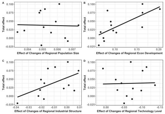
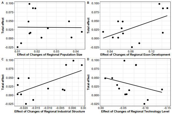
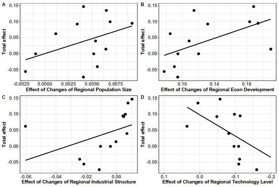
 Figure 1 Changes of regional average CEI
 Table 1 Inter-regional CEI differences


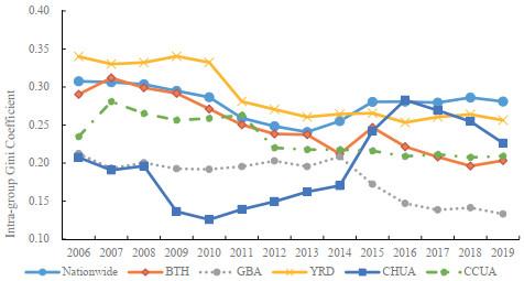

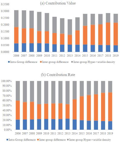
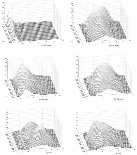
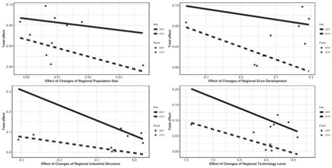
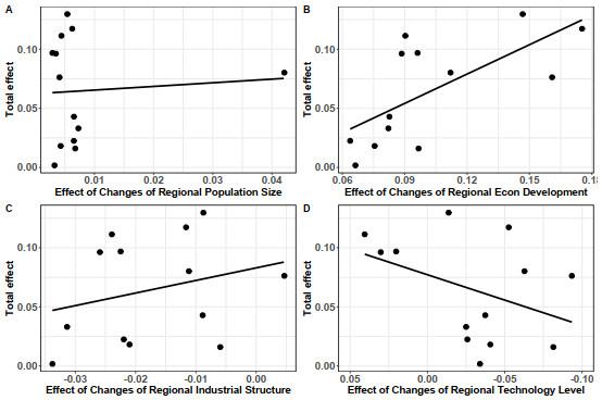
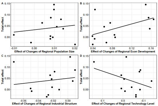
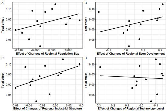
