1 Introduction
The stock market is a barometer of the economic and financial activities of a country or region, reflecting the development of the national economy. In the context of economic globalization, stock markets are susceptible to abnormal fluctuations influenced by various uncertainties such as economic, political, and public emergencies
[1]. These fluctuations often result in substantial losses for investors and can potentially affect global stock markets. For example, the outbreak of the financial crisis in 2008 and the global outbreak of COVID-19 in 2020 caused the global stock market to suffer major losses, which caused serious harm to the global economy
[2–4]. Therefore, accurately measuring the extreme tail risk of the stock market, timely capturing and predicting it dynamically, has important practical significance and policy reference value for maintaining financial stability.
In tail risk management, Value-at-Risk (VaR) and Expected Shortfall (ES) have been two of the most frequently used methods based on quantile. Specifically, VaR is defined as the maximum potential loss that may occur when holding a certain security or asset portfolio within a specified time frame under a given confidence level
[5]. While VaR possesses the benefits of a straightforward conceptual framework and easy explication, it is not without its limitations. One drawback is its exclusive reliance on the probability of extreme losses, neglecting to account for the magnitude of these losses
[6]. Furthermore, it should be noted that VaR does not satisfy the risk additivity requirement and hence lacks consistency as a risk measurement approach. Thus, under the VaR framework, the risk of a diversified asset portfolio might surpass the sum of all individual asset risks, which contradicts the widely accepted principle that diversification reduces risk. Consequently, Artzner, et al.
[7] introduced Expected Shortfall (ES) as a tail risk measurement for portfolios, denoting the expected loss below a predefined threshold (e.g., VaR) at a given risk probability level. ES provides information about the size of losses since it is defined as the conditional average loss beyond VaR. Acerbi, et al.
[8] demonstrated that ES is a consistent risk measure. However, ES is not a consistency measurement with elicitability and, therefore, cannot be evaluated through a loss function
[9]. This limitation restricts its potential as a reliable assessment standard for risk prediction. By rectifying the undesirable property of VaR and ES, which concentrate solely on the tail of the asset loss distribution, an alternative risk measure expectile has recently received increased attention
[10–14].
Expectile, proposed by Newey and Powell
[15], has two significant advantages. First, expectile emphasizes globality, as it is not only sensitive to the numerical values of extreme losses but also captures the overall information of the distribution. Second, the quadratic loss function of expectile facilitates computations while also improving estimation accuracy
[16]. Given the aforementioned advantages of expectile, Kuan, et al.
[17] adopted expectile to define a new risk measure, namely Expectile-based Value-at-risk (EVaR). In comparison to quantile-based risk measures, EVaR is more sensitive to the magnitude of tail losses as it effectively incorporates information concerning the complete distribution. Consequently, EVaR has seen increasing adoption in the field of finance in recent years
[6, 18–23]. For example, Chen
[20] investigated the theoretical and practical issues related to EVaR in comparison with VaR and CVaR. Bellini, et al.
[19] proposed conditional EVaR and discussed its properties. More recently, Jiang, et al.
[21] developed a single-index approach for modeling EVaR and established the asymptotic normality of the resultant estimators. Liu, et al.
[22] used EVaR to predict extreme financial risk, especially when the conditional mean and the conditional variance of asset returns are nonlinear.
To compute EVaR values, Taylor
[10] and Kuan, et al.
[17] proposed a Conditional Autoregressive Expectile (CARE) model, in which positive and negative lagged returns are allowed to capture asymmetric dynamic effects on tail expectiles. Subsequently, some variants of the CARE model emerged. By assuming that the error term follows an asymmetric normal distribution, Gerlach and Chen
[24] and Gerlach, et al.
[25] proposed the CARE-R and CARE-X models by incorporating realized ranges and realized volatility into tail risk forecasting, respectively. To better capture time-varying features of conditional expectiles, Xu, et al.
[6] utilized a local parametric approach to study the parameter instability of tail risk dynamics. Gerlach and Wang
[26] proposed a new model framework called Realized-CARE by incorporating a measurement equation into the conventional CARE model. Cai, et al.
[13] introduced a class of generalized conditional autoregressive expectile (GCARE) models which include the autoregressive components of lagged expectiles.
In this paper, we adopt the localizing conditional autoregressive expectile (LCARE) model proposed by Xu, et al.
[6] to measure tail risk in the Chinese stock market. We first determine homogeneous intervals through the local parametric approach (LPA) and then establish a CARE model with constant parameters within the homogeneous intervals. The reasons why we selected the LCARE model to study the Chinese stock market can be stated as follows. Firstly, the Chinese stock market is one of the largest and most dynamic stock markets in the world, making it an attractive research subject. The size and complexity of the Chinese stock market provide ample opportunities to study various aspects of stock market risks, especially market volatility. In addition, the Chinese economy has experienced rapid growth in recent years, leading to significant changes in the financial sector, which poses unique risks and challenges. The study of stock market risks in China can provide valuable insights into the relationship between economic growth and stock market performance, as well as the potential risks associated with financial sector development. Secondly, the study of stock market risks in China can offer valuable lessons for other countries, as the Chinese market serves as a bellwether for the economic and financial activities of the region. The findings from the analysis of Chinese stock market risks can be generalized to other emerging markets, helping investors and regulators better understand and manage the risks associated with stock market investments.
Thirdly, although numerous research endeavors have undertaken the task of characterizing tail risk in the Chinese stock market through the application of VaR, ES and EVaR
[27–31], very few of them have considered the dynamic changes in the tail distribution of stock market returns and the associated time-varying parameters, which may prevent the data-driven selection of dynamic change features. The LCARE model can overcome such restrictions and has the ability to fully capture potential market condition structure changes and time-varying fluctuations in the dynamic stock market. Finally, the adaptive modeling framework used in the LCARE model has been successfully applied in many econometric settings and research fields, demonstrating the enormous potential and application value of the LCARE model in tail risk measurement
[32–36]. For example, Spokoiny
[32] proposed a local change point test to detect the largest interval not containing any change for every time point, and applied it to the volatility modeling of assets. Chen and Niu
[33] and Chen, et al.
[34] proposed the adaptive DNS model to better forecast the Treasury yield curve and the term structure of option-implied volatility, respectively. Mihoci, et al.
[35] used the local adaptive technique successfully to predict financial time series, i.e. the buyer- and the seller-initiated trading volumes and the order flow dynamics. Chen, et al.
[36] unravelled the intricate network of interconnectedness and the ever-changing structural dynamics within global, regional, and intra-ASEAN markets by leveraging the innovative Adaptive Matrix Autoregressive (AMAR) model.
The contributions of this paper to the existing literature are multifaceted. Firstly, we innovatively adopt the LCARE model to locally estimate the expectile risk measure rather than following a traditional approach of assuming constant CARE parameters over the pre-given data intervals. This helps the precise measurements of tail risk exposure at different expectile levels and risk power levels and its corresponding ES at different market conditions. The lengths of the homogeneity intervals obtained through the local parametric approach provide strong evidence for the presence of potential structural changes in tail risk measurement. Secondly, we employ the wavelet transform to compare the performance of the LCARE model and CARE model at different time scales, establishing the effectiveness of the LCARE model through intuitive data. The suggested LCARE model has the potential to assist investors in making diverse investment decisions across different investment horizons. Thirdly, we apply the LCARE model to the Time-Invariant Portfolio Protection (TIPP) strategies to incorporate a time-varying risk multiplier. The empirical results demonstrate that the time-varying multiplier TIPP strategy based on LCARE exhibits enhanced performance in comparison to other strategies. Thus, this study has the potential to serve as a valuable reference for government departments and investors seeking to assess and alert to the time-varying tail risk of the stock market across various market conditions and investment horizons.
The rest of the paper is organized as follows. In Section 2, we introduce the LCARE model and the estimation method. In Section 3, we conduct empirical research on the tail risk of the Chinese stock market and analyze the performance of the LCARE model at multiple time scales. The LCARE model is applied to portfolio strategies in Section 4. Section 5 concludes the paper.
2 Model and the Estimation Method
2.1 Conditional AutoRegressive Expectile (CARE) Model
The early introduction of the idea of expectile and the application of asymmetric least squares regression (ALS) were pioneered by Newey and Powell
[15]. For a stationary time series
, the
-th expectile
of
is defined as the minimizer of the following quadratic loss function:
where represents the prudentiality level, reflecting the asymmetry of the loss function, and is the indicator function.
For analyzing stationary and weakly dependent time series data, Kuan, et al.
[17] proposed the conditional autoregressive expectile (CARE) model, which directly models the time series of returns. Specifically, the CARE model is introduced as follows:
where and denote the expectile and the error term at the prudentiality level and time , respectively. Here, and denote the observed positive and negative one-period lagged returns at time , respectively. It is crucial to identify the asymmetric impact of positive and negative returns when explaining dynamic tail risk. The expectile in Eq. (2) can be estimated by minimizing the asymmetric least square loss function in Eq. (1).
Within the CARE framework, Gerlach and Chen
[24, 25] assumed that the error term
follows the asymmetric normal distribution (AND). Xu, et al.
[6] assumed that the data process follows an asymmetric normal distribution
conditionally on the information set
, with the probability density function:
where is the expectile loss function, represents the expectile value to be estimated, and represents the variance of the error term. It can be proven that maximizing the likelihood based on the distribution of Eq. (4) is equivalent to minimizing the asymmetric least square loss function in Eq. (1).
Conditional on the information set up to observation , the expectile includes a one-period lagged return component, which can mimic volatility clustering in financial series and potential asymmetric magnitude effects. In Eq. (3), the parameter vector is , where and explain the asymmetric impact on the conditional tail expectile magnitude of positive and negative lagged returns. This similarly mimics the leverage effect of return volatility, where negative (positive) returns are followed by relatively higher (lower) volatility.
The quasi-log-likelihood function for observed data in a fixed interval is:
For the observation on a right-end fixed interval of observations, the quasi maximum likelihood estimate (QMLE) of CARE parameters is obtained through:
Let represent the pseudo-true parameter vector at prudentiality level . The quality of the estimation given in Eq. (6) can be measured by the Kullback-Leibler (KL) divergence:
where
is the risk bound and
denotes the risk level. More details about parameters can be found in [
16].
2.2 Localizing Conditional Autoregressive Expectile (LCARE) Model
In time series, longer data intervals can lead to larger modeling bias, while shorter intervals can result in more unstable parameters. The LCARE model integrates the Local Parametric Approach proposed by Spokoiny
[16] and the CARE model introduced by Kuan, et al.
[17]. The basic idea is to find the longest data interval, i.e., the homogeneous interval, over which a CARE model with time-invariant parameters can be well established. Through a sequential test, the so-called local change point detection test can adaptively select the homogeneous interval within the candidate intervals. The Monte Carlo method is used to simulate the critical values of the sequential test. Finally, based on the test results, the adaptively estimated parameter vectors can be chosen at each time point
. Please see more details in [
6].
2.2.1 The Sequential Test
The sequential test can adaptively identify homogeneous intervals at a fixed time point . Assuming interval is homogeneous, we consider the homogeneity of the interval and perform tests sequentially over the index . At step , the test hypothesis is:
: No change point in the interval ,
: Exist change point in the interval .
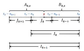
The test statistic is:
where
(dotted part in
Figure 1) and
(solid part in
Figure 1) are subintervals of
. The algorithm at step
is illustrated in
Figure 1.
Figure 1 The sequential test at a fixed time point in an interval of length |
Full size|PPT slide
If the null hypothesis about the homogeneity of the interval is not rejected, we proceed to test the homogeneity of the interval . Since the location of the change point within is unknown, the test statistic is calculated based on all points , i.e. , utilizing data from . Calculate the sum of the log-likelihood values on sample intervals and , subtract the log-likelihood value on , and then use Eq. (8) to determine the test statistic at each predetermined expectile level .
To identify the length of the homogeneous interval, the test statistic is compared to the corresponding simulation critical value at each step (see Subsection 2.2.2 for the explanation of critical value). If all test statistics up to step do not exceed the critical value, the null hypothesis that is homogeneous is not rejected, and the test proceeds to the next step. Conversely, if the test statistic at step first exceeds the corresponding critical value, is selected as the final choice. Denote the index of the final choice of the homogeneous interval as . If the null hypothesis is already rejected in the interval , and if the null hypothesis is not rejected in the interval , . Formally, the adaptive estimate is obtained by , with .
2.2.2 Determination of Critical Values
The critical value defines the significance level of the test statistic in Eq. (8). In classical hypothesis testing, the critical values are chosen to ensure a given level of the test, i.e., the maximum probability of rejecting the null hypothesis when it is true (i.e., the probability of committing Type Ⅰ error). In the LCARE framework, critical values are used to control the loss associated with detecting a non-existent change point.
Under the null hypothesis of constant parameters, the expected homogeneous interval is the longest . When the selected interval is relatively shorter, it can effectively detect a non-existent change point, causing a ‘false alarm’. Therefore, it's necessary to control the loss associated with selecting an adaptive estimate rather than .
The critical value sequence essentially controls the threshold of the likelihood ratio test statistic in Eq. (8). However, the true distribution of the test statistic is unknown, necessitating the utilization of the Monte Carlo approach to ascertain the critical values.
For each step , the calculation is done based on the following propagation condition:
where , is the given probability level. This propagation condition of Eq. (9) controls the frequency and explains the bias of the adaptive estimates against the unknown true parameters. If the likelihood loss on the left-hand side of Eq. (9) is relatively small, it indicates a high probability that the adaptive estimate lies in the confidence set of the optimal parameter within the interval . Conversely, a large bias suggests a small probability that the adaptive estimate falls within the confidence set of the optimal estimate, i.e., differs significantly from, and there is a possible change point within the interval .
3 Empirical Study
3.1 Data and Descriptive Statistics
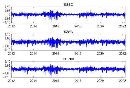
In this paper, we consider three representative stock indices: The Shanghai Composite Index (SSEC), the Shenzhen Composite Index (SZSC), and the CSI 300 Index. Daily index returns are obtained from the Wind China Financial Database, encompassing a sample period of 2, 491 trading days from 4 January 2012 to 6 April 2022. Daily returns are calculated by
where is the daily return at time , and is the closing price at time .
Figure 2 depicts the trends of daily returns for the selected three stock indices over time. Notably, there were significant fluctuations in daily returns during the stock market crash of 2015–2016. Furthermore, the changes in daily returns show the phenomenon of volatility clustering.
Figure 2 Daily returns for the SSEC, SZSC and CSI 300 series from 4 January 2012 to 6 April 2022 |
Full size|PPT slide
Table 1 provides descriptive statistics for the daily return series of the three stock indices. All three stock indices have high peaks and fat tails, as evidenced by the kurtosis and skewness indices. The Jarque-Bera (J-B) statistics significantly exceed the critical value at the 1% significance level, indicating that the daily returns are non-normal. The results of the Ljung-Box autocorrelation test suggest that there is a significant serial correlation at the 1% significance level for all three indices. Additionally, it can be observed that the return time series exhibits stationarity, as indicated by the results of the Augmented Dickey-Fuller (ADF) test. Hence, the methodology employed in this study can be utilized for modeling and analysis.
Table 1 Descriptive statistics of daily returns for the three stock indices |
| Index | SSEC | SZSC | CSI 300 |
| Mean | 0.0002 | 0.0004 | 0.0002 |
| Median | 0.0006 | 0.0013 | 0.0004 |
| Minimum | 0.0887 | 0.0879 | 0.0915 |
| Maximum | 0.0560 | 0.0632 | 0.0650 |
| Standard Dev. | 0.0133 | 0.0160 | 0.0144 |
| Skewness | 0.9950 | 0.8694 | 0.7145 |
| Kurtosis | 10.1183 | 6.8499 | 8.4609 |
| J-B Statistic | 5667.9(0.000) | 1851.4(0.000) | 3305.9(0.000) |
| Q(10) | 35.371(0.000) | 24.195(0.007) | 34.654(0.000) |
| ADF | 47.884(0.000) | 46.781(0.000) | 48.369(0.000) |
| Note: Values in parentheses indicate p-values; Q(10) denotes the 10th-order autocorrelation Ljung-Box Q statistic of daily returns. |
3.2 Necessity of the Adaptive Interval Selection
In this section, we implement a fixed rolling window exercise in order to investigate the impact of varying time intervals on modeling bias and parameter volatility, as well as to illustrate the necessity of adaptive time interval selection. We consider different interval lengths (e.g., 20 and 125 observations) and analyze the corresponding estimates. More specifically, the CARE model is trained on the selected stock indices using fixed rolling windows consisting of 20 and 125 observations, respectively. The estimated CARE parameters, denoted as
at the expectile level
, and their corresponding kernel density plots are presented in
Figure 3 and
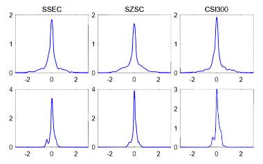
Figure 4, respectively, spanning from 2 January 2014 to 6 April 2022. The upper (lower) panel in each figure shows the estimated parameter values with a fixed rolling window of 20 (125) observations.Figure 3 Estimated parameter of the selected stock indices using fixed rolling windows of 20 (upper panel) and 125 (lower panel) observations at expectile level |
Full size|PPT slide
Figure 4 Kernel density plots for estimated parameter of the selected stock indices using fixed rolling windows of 20 (upper panel) and 125 (lower panel) observations at expectile level |
Full size|PPT slide
The volatility of parameter estimates is seen to be larger when fitting data over shorter periods in comparison to utilizing longer time intervals, as depicted in
Figure 3.
Figure 4 displays kernel density plots, employing an Epanechnikov kernel, to illustrate the estimated parameters. The findings also indicate that shorter intervals are associated with increased variability of the estimates, whereas longer intervals exhibit the opposite trend. The densities exhibit substantial differences between the two examples, with 20 observations in one case and 125 observations in the other.
Figure 5 illustrates how the direction of modeling bias varies inversely with parameter volatility. Modeling bias is lower when fitting data within shorter intervals. The blue solid line in
Figure 5 represents the expectiles
of the three stock indices obtained using the CARE model through fixed rolling windows at expectile level
. The gray solid line represents the daily returns of these three stock indices.
Figure 5 Expectiles of the selected stock indices using fixed rolling windows with 20 (upper panel) and 125 (lower panel) observations at expectile level |
Full size|PPT slide
The fixed rolling window exercise with 20 and 125 observations confirms that there exists a variance-bias trade-off in the selection of time intervals in the CARE model. A relatively shorter time interval can result in reduced modeling bias and increased parameter volatility. Therefore, the application of an adaptive method for interval selection becomes necessary. In the following part, we perform the adaptive window selection between data intervals covering 20 to 125 observations.
3.3 Adaptive Selection of Homogeneous Intervals
It should be noted that there exists a multitude of potential homogeneous intervals that may be considered as candidates. In order to reduce the computational load, we select
nested intervals of length
, i.e.,
. Following Chen and Spokoiny
[37] and Xu, et al.
[6], the set-up of the intervals is fixed as
with
and
. We also restrict the largest interval length
. This means the interval length increases at a geometric rate of
, starting from 20 observations and ending with 125 observations. To be more specific, we consider the interval set
. Additionally, it is assumed that the model parameters remain constant in the initial interval
.
3.3.1 Simulated Critical Values
The LCARE model framework requires a set of simulated critical values that depend on reasonable parameter constellations. In this paper, we adopt a data-driven approach for selecting ‘true’ parameters. The method uses the parameters estimated from the CARE model based on a sample window covering half a year, i.e., 125 observations.
Table 2 provides the estimated parameters of the three stock indices from 2 January 2014 to 6 April 2022 (a total of 2010 trading days) at two expectile levels and
, respectively. The parameters are separated into three categories: Low, mid, and high based on quartiles, corresponding to 0.25, 0.50, and 0.75 quantiles. At a given expectile level
, there are three pseudo-true parameter constellations, i.e., the parameter values most likely to be found in practice.
Table 2 Descriptive statistics of the estimated CARE parameters based on a half-year sample window, for the three stock indices from 2 January 2014 to 6 April 2022 (a total of 2010 trading days) under two expectile levels and |
| quartiles | | | |
| 0.25 | 0.50 | 0.75 | | 0.25 | 0.50 | 0.75 |
| 0.0008 | 0.0001 | 0.0008 | | 0.0008 | 0.0001 | 0.0008 |
| 0.0496 | 0.0271 | 0.1345 | | 0.0474 | 0.0001 | 0.1362 |
| 0.1074 | 1.4201 | 1.6237 | | 0.1384 | 1.4109 | 1.6299 |
| 0.0047 | 1.6173 | 4.6063 | | 0.0046 | 1.6443 | 4.6438 |
| 0.0001 | 0.0003 | 0.0003 | | 0.00010 | 0.0003 | 0.0003 |
For each pseudo-true parameter vector at a given expectile level in
Table 2, we simulated 1000 sample paths using the corresponding CARE specification. The risk bound for each vector is obtained by calculating the maximum average value of the (
th power) difference between the respective log-likelihood values, following Eq. (7). Note that the risk power level
governs the tightness of the risk bounds, leading to varying risk bounds and critical values for different level
, consequently resulting in distinct adaptive estimated intervals. Therefore, we consider the moderate risk case (
) and the relatively conservative risk case (
) at two expectile levels
and
.
Table 3 provides the values of the simulated risk bounds
across different setups. The results indicate that under conservative risk conditions, the risk boundaries are significantly larger than those under moderate risk conditions.
Table 3 Simulated risk bounds at different expectile levels and risk power levels |
| quartiles | | | |
| 0.25 | 0.50 | 0.75 | | 0.25 | 0.50 | 0.75 |
| 0.390 | 0.844 | 0.290 | | 0.430 | 0.508 | 0.525 |
| 1.689 | 5.629 | 1.518 | | 1.928 | 2.548 | 2.688 |
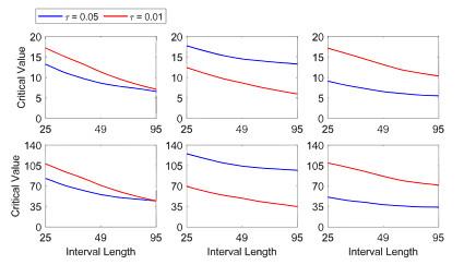
Figure 6 depicts the critical value curves for the six pseudo-true parameter vectors selected from
Table 2 and associated risk bounds from
Table 3. The upper (lower) panel represents critical values at risk power level
(
). The blue and red lines represent the expectile levels
and
respectively. It is presented that the critical values vary in a decreasing manner and exhibit a similar rate of decline across different setups. Thus, selecting a set of critical values in a data-driven fashion is rational. At a fixed time point, the estimate
derived from a half-year sample window serves as a benchmark to choose the appropriate critical value curve. For instance, if the value is below the 0.25th quantile reported in
Table 2, the leftmost panel of the critical value curve in
Figure 6 is chosen. Conversely, if the value is above the 0.75th quantile reported in
Table 2, the rightmost panel of the critical value curve in
Figure 6 is selected.
Figure 6 Simulated critical value curves for the selected six pseudo-true parameter vectors from Table 2 at the risk power level (upper panel) and (lower panel). The blue and red lines represent the expectile levels and respectively |
Full size|PPT slide
3.3.2 Homogeneous Intervals
The sequential local change point detection test is used to determine the optimal length of homogeneous intervals at different expectile levels. The probability level
is set at 0.05.
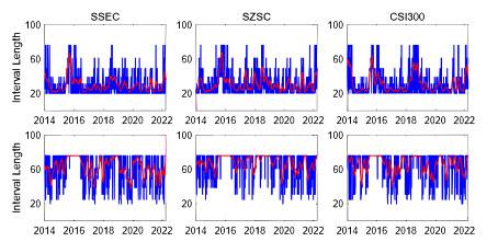
Figure 7 and
Figure 8 display the estimated lengths of homogeneous intervals for the three stock indices from 2 January 2014 to 6 April 2022 at expectile levels and
respectively. The upper panel depicts the moderate risk case
, whereas the lower panel denotes the conservative risk case
. The blue lines represent the estimated lengths of homogeneous intervals, while the red lines denote the smoothed values of intervals with a length of 20 days (one month). It indicates that after the 2015 stock market crash, there were relatively longer homogeneous intervals. Influenced by the COVID-19 pandemic, the intervals became shorter after 2020. It is noteworthy that the primary objective of the LCARE model is to identify the longest intervals of homogeneity in which the null hypothesis of CARE parameters is not rejected. During periods characterized by significant market events such as the 2015 stock market crash and the COVID-19 pandemic, the homogeneous intervals tend to be shorter because of the increasing market volatility and obvious market turmoil. During the period subsequent to these events, the homogeneous intervals exhibit comparatively longer.
Figure 7 Estimated lengths of homogeneous intervals for the three stock indices from 2 January 2014 to 6 April 2022 at expectile level . The upper panel depicts the moderate risk case , whereas the lower panel denotes the conservative risk case |
Full size|PPT slide
Figure 8 Estimated lengths of homogeneous intervals for the three stock indices from 2 January 2014 to 6 April 2022 at expectile levels . The upper panel depicts the moderate risk case , whereas the lower panel denotes the conservative risk case |
Full size|PPT slide
Table 4 provides the average daily optimal interval length of the three selected stock indices at different levels of expectile and risk power. It turns out that compared with the conservative risk case
, the homogeneous intervals in the moderate risk case
are relatively shorter. In addition, the intervals of homogeneity at expectile level
are slightly shorter than the intervals at
.
Table 4 Average daily optimal interval length for the three stock indices at different expectile levels and risk power levels |
| | | | |
| SSEC | SZSC | CSI 300 | | SSEC | SZSC | CSI 300 |
| 44 | 42 | 46 | | 29 | 31 | 31 |
| 72 | 73 | 72 | | 62 | 68 | 66 |
3.4 Dynamic Tail Risk Exposure
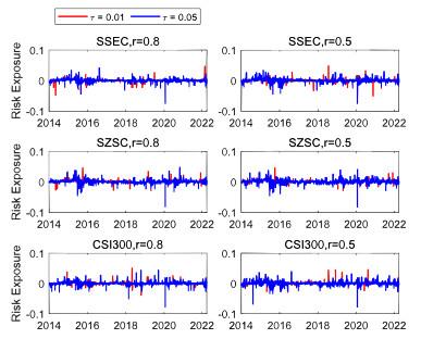
In this section, the dynamic tail risk exposure of the selected stock indices is estimated by using the adaptively selected homogeneous intervals.
Figure 9 illustrates the estimated tail risk exposure for the three stock indices from 2 January 2014 to 6 April 2022 based on the LCARE model at different expectile levels and risk power levels. The left panel represents the results of the conservative risk case , whereas the right panel considers the moderate risk case
. Notably, under moderate risk, the tail risk exposure exhibits slightly higher variability on average, which results in shorter homogeneous intervals as shown in
Table 4.
Figure 9 Estimated tail risk exposure for the three stock indices from 2 January 2014 to 6 April 2022 at expectile level (blue) and (red). The left panel represents the results of the conservative risk case , whereas the right panel considers the moderate risk case |
Full size|PPT slide
Additionally, expected shortfall (ES) can be calculated using the estimated expectiles. According to Taylor
[10], there is a one-to-one mapping between quantiles and expectiles. To equate expectile
with the expectile level
to
-quantile
, i.e.,
, the following equation is used:
where is the cumulative distribution function of a random variable , in this paper we consider the asymmetric normal distribution. The corresponding ES can be expressed as:
with denoting the expectile at the level .
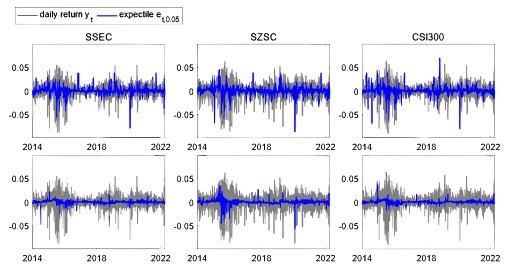
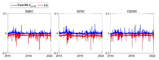
Figure 10 displays the expectiles (blue solid line) and ES (red solid line) for the three stock indices at expectile level
and risk power level
. During market downturns, such as the 2015 Chinese stock market crash, the 2018 Sino-US trade friction, and the 2020 COVID-19 pandemic, the estimated ES exhibits a high variability. Similarly to current research developments, the estimated ES using the proposed LCARE model exceeds (by magnitude) the estimated expectile
value.
Figure 10 Expectiles (blue) and expected shortfall (red) for the three stock indices at expectile level and risk power level |
Full size|PPT slide
3.5 Performance Analysis of the LCARE Model at Multiple Time Scales
Since Grossmann and Morlet
[38] first introduced the wavelet transform theory, wavelet transform has been used for analyzing strategies with different investment horizons. It aims to assist investors with diverse purposes in diversifying their investments more reasonably during periods of market volatility, thereby reducing the potential for losses
[39]. To study the predictive performance of the LCARE model at different time scales, we employ the Maximal Overlap Discrete Wavelet Transform (MODWT) to decompose the daily return series
[40]. For a time series signal
of length
, the scale coefficients
and wavelet coefficients
in MODWT can be represented as follows:
where and are -dimensional vectors, and represent the scaling and wavelet filters for the th level, with being the filter length. In this paper, we select a Least Asymmetric filter with a filter length of 8. At the th level scale, the corresponding frequency range is . When the time interval is , the corresponding period for the th level scale is given by .
Denoting the original time series as
, we apply the MODWT method to decompose the daily return series of the Shanghai Composite Index (SSEC), Shenzhen Composite Index (SZSC), and the CSI 300 Index. The different components are denoted from high to low frequency as
,
,
, corresponding to time scales of
,
and
days respectively. For model fitting, the dataset utilized in this section spans from January 4, 2021, to April 6, 2022, covering a total of 303 trading days. The loss function values for Eq. (1) are obtained and compared with the loss function values of the CARE model under different rolling windows, as shown in Table 5. It is evident that, at different expectile levels, the LCARE model consistently exhibits lower loss function values, with superior predictive performance at the
days frequency.
Table 5 The loss function values of the CARE model and LCARE model at different time scales |
| | | | |
| Rolling window of CARE | | LCARE | | Rolling window of CARE | | LCARE |
| 20 | 60 | 125 | | | | | 20 | 60 | 125 | | | |
| SSEC |
| 0.0232 | 0.0187 | 0.0180 | | 0.0148 | 0.0172 | | 0.0219 | 0.0176 | 0.0177 | | 0.0140 | 0.0139 |
| 0.0087 | 0.0069 | 0.0067 | | 0.0064 | 0.0076 | | 0.0086 | 0.0069 | 0.0063 | | 0.0084 | 0.0086 |
| 0.0032 | 0.0037 | 0.0039 | | 0.0073 | 0.0070 | | 0.0033 | 0.0037 | 0.0039 | | 0.0079 | 0.0045 |
| 0.0012 | 0.0016 | 0.0018 | | 0.0029 | 0.0012 | | 0.0042 | 0.0034 | 0.0018 | | 0.0042 | 0.0011 |
| SZSC |
| 0.0369 | 0.0251 | 0.0279 | | 0.0235 | 0.0269 | | 0.0381 | 0.0267 | 0.0275 | | 0.0222 | 0.0236 |
| 0.0107 | 0.0108 | 0.0095 | | 0.0106 | 0.0100 | | 0.0113 | 0.0110 | 0.0100 | | 0.0136 | 0.0100 |
| 0.0055 | 0.0065 | 0.0059 | | 0.0067 | 0.0063 | | 0.0063 | 0.0065 | 0.0069 | | 0.0066 | 0.0069 |
| 0.0021 | 0.0032 | 0.0034 | | 0.0066 | 0.0032 | | 0.0040 | 0.0040 | 0.0040 | | 0.0044 | 0.0044 |
| CSI 300 |
| 0.0247 | 0.0294 | 0.0299 | | 0.0246 | 0.0232 | | 0.0262 | 0.0289 | 0.0293 | | 0.0257 | 0.0230 |
| 0.0123 | 0.0109 | 0.0107 | | 0.0110 | 0.0122 | | 0.0112 | 0.0122 | 0.0119 | | 0.0132 | 0.0121 |
| 0.0050 | 0.0061 | 0.0060 | | 0.0050 | 0.0067 | | 0.0050 | 0.0059 | 0.0060 | | 0.0069 | 0.0078 |
| 0.0030 | 0.0030 | 0.0029 | | 0.0016 | 0.0030 | | 0.0030 | 0.0029 | 0.0029 | | 0.0033 | 0.0026 |
4 Application of LCARE in Portfolio Strategies
Dynamic tail risk measurement is a valuable tool in quantitative finance. For instance, portfolio insurance strategies aim to ensure a minimum wealth level over a given time horizon while considering the potential returns of the portfolio. Existing generic strategies and variations include Option Based Portfolio Insurance (OBPI), Constant Proportion Portfolio Insurance (CPPI), and Time-Invariant Portfolio Protection (TIPP) strategies.
The OBPI strategy, introduced by Leland and Rubinstein
[41], replicates options by adjusting the allocation between stocks and risk-free assets to achieve capital protection. Investors employing this strategy buy put options while holding risk assets such as stocks, allowing them to benefit from the price rise of risk assets and lock in the maximum loss in case of price falls. The CPPI strategy proposed by Black and Jones
[42] divides the investment capital into two parts: One invested in risk-free assets to ensure a certain proportion of the capital remains unaffected by market risk, while the other invested in risk assets to participate in market volatility and seek potential returns. Estep and Kritzman
[43] made modifications to the CPPI strategy, introducing the TIPP strategy. It allows for the variation of the protection amount, linking the insurance amount to the portfolio value. The insurance amount is set as a fixed proportion of the highest portfolio value at any given time point. When the portfolio value changes, a new insurance amount is calculated, and the larger of the new and previous insurance amount is selected as the post-net asset value insurance amount. Therefore, the insurance adjustment of the TIPP strategy, which only increases and does not decrease, adequately reflects the continuous updating of investment costs, rather than arbitrary historical costs. The TIPP strategy has received continuous attention since its proposal, and some literature has discussed its performance and made improvements to it
[44–48]. For example, Li, et al.
[44] found the most optimized multiplier of TIPP in various situations via an artificial neural network so as to optimize dynamic portfolio insurance. Hamidi, et al.
[45] introduced a dynamic autoregressive expectile approach for the TIPP conditional multiple. The empirical results of Mancinelli and Oliva
[47] showed that TIPP outreaches CPPI regarding downside protection, even though it cannot face potential upside capture. Di Persio, et al.
[48] proposed to modify the standard TIPP strategy by adding an investment threshold in the risky asset allocation.
The TIPP strategy can be expressed as:
where represents the total value of the portfolio at time , denotes the maximum investment value in risk assets at time , is the minimum value of the investment in risk-free assets at time , represents the risk multiplier for the portfolio, indicates the capital protection floor of the portfolio at time , denotes the capital protection ratio at time , reflects the annual return of the risk-free asset, and is the investment horizon.
The proportion of the total portfolio value invested in risk assets is determined by the risk multiplier, which represents the risk exposure of the portfolio. Traditional methods often assume that the multiplier is a constant, i.e., insensitive to current market conditions.
Figures 11 and
12 respectively show the performance of the TIPP strategy with different risk multipliers applied to the Shenzhen Composite Index in bull and bear markets. It can be observed that selecting a larger risk multiplier is beneficial for outperforming the market in an uptrend while opting for a lower risk multiplier can limit associated losses in a downtrend.
Figure 11 Performance of the TIPP strategy with different risk multipliers on the Shenzhen Component Index (SZSC) during a bull market |
Full size|PPT slide
Figure 12 Performance of the TIPP strategy with different risk multipliers on the Shenzhen Component Index (SZSC) during a bear market |
Full size|PPT slide
In the TIPP strategy, it is assumed that market asset prices change continuously and can be traded without cost, avoiding the situation where the guarantee of returns cannot be cashed in at maturity. However, unpredictable large-scale downward market movements may occur in practice, where investors cannot reallocate their portfolio configurations during discontinuous rebalancing. Therefore, investors must consider the risk of unfulfilled capital protection at the maturity date, known as gap risk. Föllmer and Leukert
[49] proposed using quantile hedging to address gap risk and calculate the multiplier accordingly. Since quantile techniques find it challenging to consider the magnitude of tail risk, Expected Shortfall (ES) as a coherent risk measure is more suitable for reflecting tail risk. Therefore, Hamidi, et al.
[45] suggested using ES to estimate the risk multiplier when investors prefer a more conservative asset allocation.
As previously stated, the Expectile-based Value at Risk (EVaR) method possesses certain advantages in comparison to the Value at Risk (VaR) and Expected Shortfall (ES) approaches when assessing tail risk. Hence, the LCARE model is employed to predict the ES to manage gap risk, leading to the derivation of risk multipliers that vary over time. One key benefit of this technique lies in its ability to dynamically alter risk multipliers based on risk assessment, eliminating the requirement for pre-selection and fixing. In advantageous circumstances, a greater proportion of resources can be assigned to investments with higher levels of risk, and conversely, in less favorable situations, a smaller proportion of resources can be given to such investments. The estimation of the risk multipliers based on LCARE is given by:
where
represents the corresponding expectile. Typically, the data is assumed to follow an asymmetric normal distribution. The threshold range is set as
.
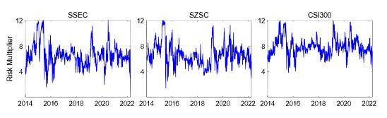
Figure 13 shows the time-varying multipliers corresponding to the ES estimates based on the LCARE model.
Figure 13 Time-varying multipliers corresponding to the ES estimates based on LCARE |
Full size|PPT slide
Assuming an initial portfolio value of 100 and a capital protection ratio of 0.9, the asset allocation decision at time
is to invest the difference between the portfolio value and the breakeven point at time
multiplied by the risk multiplier in risk assets, with the remainder invested in risk-free assets.
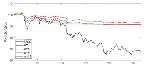
Figure 14 depicts the performance of different portfolio insurance strategies. It can be observed that both the time-varying multiplier TIPP strategy based on LCARE and the fixed multiplier TIPP strategy outperform the OBPI strategy. Within the TIPP strategy, the time-varying multipliers are more adept at capturing changes in market conditions compared to the fixed multipliers. Overall, the TIPP method, which is based on the LCARE framework and incorporates a time-varying multiplier, demonstrates superior performance compared to other strategies.
Figure 14 Performance of portfolio insurance strategies. (Black line: observed stock index; Red line: time-varying multiplier TIPP strategy based on LCARE; Green line: TIPP strategy with a fixed multiplier ; Blue line: time-varying multiplier TIPP strategy based on CARE with half-year fixed rolling window; Purple line: synthetic put strategy) |
Full size|PPT slide
Table 6 lists the descriptive statistics of portfolio returns for different strategies. For different stock indices, the time-varying multiplier TIPP strategy based on LCARE has the highest annualized return compared to other benchmark strategies. Although its annualized volatility is lower than the synthetic put strategy, it is higher than both the time-varying multiplier TIPP strategy based on the CARE model with a half-year fixed rolling window and the fixed multiplier TIPP strategy. It suggests that the LCARE model effectively balances the modeling bias and parameter volatility. Furthermore, it is worth noting that the LCARE-based strategy exhibits the highest Sharpe ratio when compared to the other strategies, implying this particular strategy offers the most favorable risk-adjusted return.
Table 6 Average daily optimal interval length for the three stock indices at different expectile levels and risk power levels |
| | Return(%) | Volatility(%) | VaR 99% | Skewness | Kurtosis | Sharpe |
| SSEC |
| SSEC | 5.46 | 21.70 | 13.22 | 1.13 | 10.47 | 0.02 |
| LCARE | 15.20 | 10.7 | 4.13 | 0.60 | 26.25 | 0.09 |
| CARE: Half year | 7.45 | 8.16 | 2.90 | 2.74 | 65.92 | 0.06 |
| Multiplier 12 | 6.33 | 8.10 | 3.38 | 2.81 | 68.39 | 0.05 |
| Synthetic put | 3.40 | 19.30 | 11.69 | 1.23 | 11.04 | 0.01 |
| SZSC |
| SZSC | 8.70 | 25.85 | 14.40 | 0.96 | 7.20 | 0.02 |
| LCARE | 11.81 | 8.22 | 3.57 | 0.56 | 22.37 | 0.09 |
| CARE: Half year | 11.08 | 7.57 | 3.03 | 0.67 | 32.68 | 0.09 |
| Multiplier 12 | 9.24 | 8.21 | 11.76 | 0.37 | 31.23 | 0.07 |
| Synthetic put | 6.17 | 23.33 | 13.35 | 1.03 | 7.58 | 0.02 |
| CSI 300 |
| CSI 300 | 7.52 | 23.07 | 12.26 | 0.86 | 8.98 | 0.02 |
| LCARE | 11.39 | 9.32 | 3.76 | 0.01 | 32.37 | 0.08 |
| CARE: Half year | 6.57 | 7.75 | 2.93 | 1.91 | 76.13 | 0.05 |
| Multiplier 12 | 5.16 | 7.78 | 3.24 | 2.48 | 78.44 | 0.04 |
| Synthetic put | 5.28 | 20.54 | 11.33 | 0.93 | 9.08 | 0.02 |
5 Conclusion
This study applies the localizing conditional autoregressive expectiles (LCARE) model to provide a comprehensive and innovative measure of the dynamic tail risk in the Chinese stock market. Empirical results show that the incorporation of time-varying parameter characteristics and potential market condition structure changes in the LCARE model enables it to effectively and precisely detect homogeneous volatility intervals, particularly the short intervals of intense volatility observed during stock market crashes. The precise measurements of tail risk exposure at different expectile levels and risk power levels and its corresponding expected shortfall (ES) at different market conditions can be calculated. Furthermore, the LCARE model is proven to improve insurance strategies well, especially the Time-Invariant Portfolio Protection (TIPP) strategies. The TIPP strategy, which is grounded in the LCARE framework and incorporates a time-varying multiplier, exhibits enhanced performance in comparison to other strategies.
It also offers decision-making insights for regulatory authorities in formulating effective financial policies and for investors in mitigating financial risks. The policy implications derived from our study are as follows. First, regulatory authorities should dynamically adjust regulatory strategies according to market conditions when monitoring extreme tail risks in the stock market. Simultaneously, the construction of a tail risk measurement system tailored to the specific conditions of China is crucial. The Expected Shortfall (ES) dynamically estimated by the LCARE model can serve as a pivotal reference indicator. Second, investors, while focusing on the inherent risks of the financial market, need to invest rationally, dynamically optimize asset allocation and portfolio insurance, and effectively guard against financial risks.
In future research, it can be considered to apply the bootstrap technique to the adaptive modeling framework, simulating the critical values by a multiplier bootstrap technique. By doing so, the assumption that the error term follows the asymmetric normal distribution can be avoided. In addition, applying the local parameter approach to the factor model would also be an interesting research direction.
{{custom_sec.title}}
{{custom_sec.title}}
{{custom_sec.content}}
 PDF(3766 KB)

 ), Yuhan MA1(
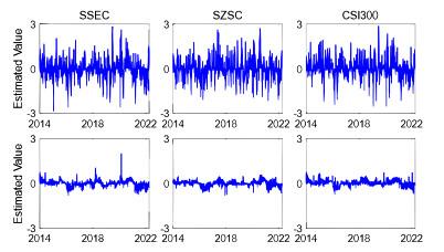
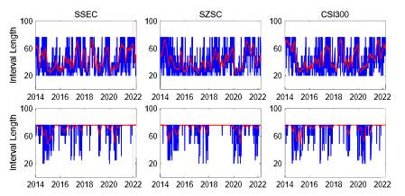
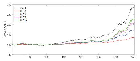
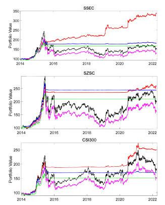
 Figure 1 The sequential test at a fixed time point
  Table 1 Descriptive statistics of daily returns for the three stock indices


