 PDF(545 KB)

A High-Moment Trapezoidal Fuzzy Random Portfolio Model with Background Risk
Xiong DENG, Yanli LIU
Journal of Systems Science and Information ›› 2018, Vol. 6 ›› Issue (1) : 1-28.
PDF(545 KB)
PDF(545 KB)
A High-Moment Trapezoidal Fuzzy Random Portfolio Model with Background Risk
In most exiting portfolio selection models, security returns are assumed to have random or fuzzy distributions. However, uncertainties exist in actual financial markets. Markets are associated not only with inherent risk, but also with background risk that results from the differences among individual investors. This paper investigated the compliance of stock yields to the fuzzy-natured high-order moments of random numbers in order to develop a high-moment trapezoidal fuzzy random portfolio risk model based on variance, skewness, and kurtosis. Data obtained from the Shanghai Stock Exchange and Shenzhen Stock Exchange was used to assess the influence on the proposed model of both background risk and the maximum level of satisfaction of the portfolio. The empirical results demonstrated that the differences between the maximum and minimum variance, skewness, and kurtosis values of the portfolio were positively correlated with the variance of the background risk.
background risk / fuzzy random number / kurtosis / portfolio selection / satisfaction / skewness {{custom_keyword}} /
Table 1 The year-to-date return ratio and variance of the eight stocks |
| Stock | Year return ratio | Variance |
| 900941 | 0.0561 | 0.1844 |
| 900943 | 0.0558 | 0.2725 |
| 900945 | 0.1595 | 0.4949 |
| 900948 | 0.0583 | 0.4744 |
| 900949 | 0.1019 | 0.3422 |
| 900950 | 0.1002 | 0.4464 |
| 900956 | 0.0880 | 0.3478 |
| 900957 | 0.0773 | 0.3468 |
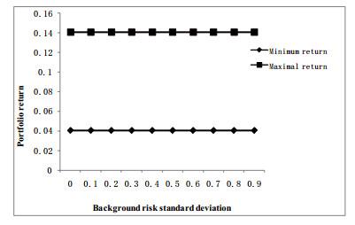
Figure 1 Relationship between the standard deviation from background risk and portfolio return |
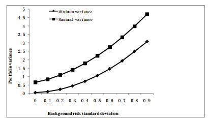
Figure 2 Relationship between the standard deviation from background risk and portfolio variance |
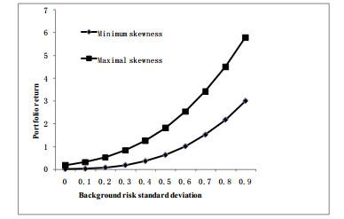
Figure 3 Relationship between the standard deviation from background risk and portfolio skewness |
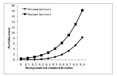
Figure 4 Relationship between the standard deviation from background risk and portfolio kurtosis |
| 1 |
{{custom_citation.content}}
{{custom_citation.annotation}}
|
| 2 |
{{custom_citation.content}}
{{custom_citation.annotation}}
|
| 3 |
{{custom_citation.content}}
{{custom_citation.annotation}}
|
| 4 |
{{custom_citation.content}}
{{custom_citation.annotation}}
|
| 5 |
{{custom_citation.content}}
{{custom_citation.annotation}}
|
| 6 |
{{custom_citation.content}}
{{custom_citation.annotation}}
|
| 7 |
{{custom_citation.content}}
{{custom_citation.annotation}}
|
| 8 |
{{custom_citation.content}}
{{custom_citation.annotation}}
|
| 9 |
{{custom_citation.content}}
{{custom_citation.annotation}}
|
| 10 |
{{custom_citation.content}}
{{custom_citation.annotation}}
|
| 11 |
{{custom_citation.content}}
{{custom_citation.annotation}}
|
| 12 |
{{custom_citation.content}}
{{custom_citation.annotation}}
|
| 13 |
{{custom_citation.content}}
{{custom_citation.annotation}}
|
| 14 |
{{custom_citation.content}}
{{custom_citation.annotation}}
|
| 15 |
{{custom_citation.content}}
{{custom_citation.annotation}}
|
| 16 |
{{custom_citation.content}}
{{custom_citation.annotation}}
|
| 17 |
{{custom_citation.content}}
{{custom_citation.annotation}}
|
| 18 |
{{custom_citation.content}}
{{custom_citation.annotation}}
|
| 19 |
{{custom_citation.content}}
{{custom_citation.annotation}}
|
| 20 |
{{custom_citation.content}}
{{custom_citation.annotation}}
|
| 21 |
{{custom_citation.content}}
{{custom_citation.annotation}}
|
| 22 |
{{custom_citation.content}}
{{custom_citation.annotation}}
|
| 23 |
{{custom_citation.content}}
{{custom_citation.annotation}}
|
| 24 |
{{custom_citation.content}}
{{custom_citation.annotation}}
|
| 25 |
Briec W, Kerstens K, Ignace V D W. Risk-loving and risk-averse preferences in mean-variance-skewness-kurtosis portfolio modeling: A common characterization using the shortage function. 2013.
{{custom_citation.content}}
{{custom_citation.annotation}}
|
| 26 |
{{custom_citation.content}}
{{custom_citation.annotation}}
|
| 27 |
{{custom_citation.content}}
{{custom_citation.annotation}}
|
| 28 |
{{custom_citation.content}}
{{custom_citation.annotation}}
|
| 29 |
{{custom_citation.content}}
{{custom_citation.annotation}}
|
| 30 |
{{custom_citation.content}}
{{custom_citation.annotation}}
|
| 31 |
{{custom_citation.content}}
{{custom_citation.annotation}}
|
| 32 |
{{custom_citation.content}}
{{custom_citation.annotation}}
|
| 33 |
{{custom_citation.content}}
{{custom_citation.annotation}}
|
| {{custom_ref.label}} |
{{custom_citation.content}}
{{custom_citation.annotation}}
|
PDF(545 KB)
 Table 1 The year-to-date return ratio and variance of the eight stocks
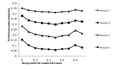
 Figure 1 Relationship between the standard deviation from background risk and portfolio returnFigure 2 Relationship between the standard deviation from background risk and portfolio varianceFigure 3 Relationship between the standard deviation from background risk and portfolio skewnessFigure 4 Relationship between the standard deviation from background risk and portfolio kurtosisFigure 5 Relationship between the standard deviation from background risk and maximum portfolio satisfaction
/
| 〈 |
|
〉 |


