Worst-Case Investment Strategy with Delay

Chunxiang A; Yi SHAO

doi:10.21078/JSSI-2018-035-23

PDF(355 KB)

Journal of Systems Science and Information ›› 2018, Vol. 6 ›› Issue (1) : 35-57. DOI: 10.21078/JSSI-2018-035-23

Worst-Case Investment Strategy with Delay

Author information +

History +

Abstract

This paper considers a worst-case investment optimization problem with delay for a fund manager who is in a crash-threatened financial market. Driven by existing of capital inflow/outflow related to history performance, we investigate the optimal investment strategies under the worst-case scenario and the stochastic control framework with delay. The financial market is assumed to be either in a normal state (crash-free) or in a crash state. In the normal state the prices of risky assets behave as geometric Brownian motion, and in the crash state the prices of risky assets suddenly drop by a certain relative amount, which induces to a dropping of the total wealth relative to that of crash-free state. We obtain the ordinary differential equations satisfied by the optimal investment strategies and the optimal value functions under the power and exponential utilities, respectively. Finally, a numerical simulation is provided to illustrate the sensitivity of the optimal strategies with respective to the model parameters.

Key words

worst-case scenario / portfolio / stochastic differential delay equation / Hamilton-Jacobi-Bellman equation / equilibrium strategies

Cite this article

EndNote

Ris (Procite)

Bibtex

Download Citations

Chunxiang A , Yi SHAO. Worst-Case Investment Strategy with Delay. Journal of Systems Science and Information, 2018, 6(1): 35-57 https://doi.org/10.21078/JSSI-2018-035-23

1 Introduction

Nowadays, an increasing number of investors do not make their portfolio decisions by themselves, but delegate their money to professional fund managers. Therefore, the fund managers and the fund investors are involved in the investment process. The fund managers can decide on the composition of the fund portfolio in light of some criteria or methods such as classic portfolio theory, and meanwhile the fund investors decide whether to invest their money to some funds or withdraw their money from the fund on basis of the investment performance of the fund managers.

As we well know, the classical portfolio theory starts from the seminal work of Markowitz^[1] on minimizing the variance with a given anticipated return or maximizing the expected returns with a given variance, i.e., Mean-Variance (M-V) model. Merton^{[2, 3]} pioneers the research of continuous-time portfolio optimization problem with the constant relative risk aversion (CRRA) utility. Later, M-V model is also extended to cases of multi-period and continuous-time setting. And from then, a substantial flow of research on the portfolio optimization problem emerges to extend previous work to different optimality criteria and different price process models for risky assets. Moreover, due to the time-inconsistency of the mean-variance criteria, a time-consistence strategy is investigated, see Björk and Murgoci^{[4, 5]}, Björk, et al.^[6] and references therein.

However, when the fund managers make their investment decisions, at least two important aspects, which is different from the classical portfolio optimization model, must be considered: A crash-threatened financial market and past preformation-related capital inflow/outflow.

On one hand, a fund manager can suffer a crash-threatened financial market such as October 1987 and September 2008, when the prices of risky assets have sudden downward movements, i.e., crashes. It is important to mention that a fund manager will undertake greater risk in a crash-threatened financial market if she makes her investment decision based on classical portfolio optimization theory. In the most of continuous-time portfolio optimization models, the prices of risky assets are assumed to follow geometric Brownian motions (GBMs), however, it is well-known that the risky assets' prices described by the GBMs are not able to explain the large price sudden downward movements (crashes). The standard approach to model crashes is to include large jumps in the dynamics of risky assets' prices possibly in addition to regular jumps of smaller size (see [7]). We refer the readers to Cont and Tankov^[8] and the references therein for an overview of financial modeling with jump processes. However, Korn and Wilmott^[9] pointed out that the jump-diffusion model only leads to strategies which hedge a crash on average over the investment horizon. In other words, the investment strategies inducing by the jump-diffusion model is not a real protection against the consequences of a crash at all. Particularly, when the large stock price crashes like October 1987 and September 2008 happen, an investor suffers large losses if she adopts the investment strategy derived from jump-diffusion model.

Based on these reasons above-mentioned, Korn and Wilmott^[9] pioneer the worst-case approach to portfolio optimization problem under the threat of a crash. Specifically, the financial market is distinguished between "crash-free state" (i.e., normal state) and "crash state". In the crash-free state the risky assets' prices behave as GMBs, and in crash state all risky assets' prices fall suddenly and simultaneously. Instead of maximizing the expected utility of terminal wealth, the worst-case bound of an investment strategy is used as optimization criterion. That is, for each admissible investment strategy, a worst-case scenario is determined and the investment strategy is considered optimal when the investment strategy yields the highest expected utility in its worst-case scenario. In fact, the investment strategy under the worst-case scenario is an equilibrium optimal strategy, so we call the equilibrium optimal strategy as optimal strategy in brief. Obviously, the pure bond strategy yields lower bounds and a poor performance if there is no crash happen at all. On the other hand, if an investor adopts the optimal investment strategies derived from the GMBs stock model, she will undertake greater risk under the threat of a crash. The worst-case model, however, arrives at a typical balance problem between obtaining good worst-case bounds for the case of a crash and also a reasonable performance if no crash occurs at all.

Korn and Wilmott^[9] studied optimal investment strategy only for a logarithmic investor with finite time horizon. Their results show that the optimal investment strategy under the threat of a crash is time-dependent and it can be determined as a solution of an ordinary differential equation. While Korn and Menkens^[10] treated a more general problem of the worst-case form by applying the dynamic programming approach. They embed the worst-case approach into the stochastic control framework. Seifried^[11] studied the worst-case portfolio problem for more general price processes by means of the martingale approach. Three literature aforementioned assumes that at most one crash can occur during the investment horizon. However, Korn and Steffensen^[12] investigated the optimal investment problem under the worst-case criterion when there happen

n (n > 1)

crashes. Their main result is a verification theorem, which asserts that a system consisting of an HJB-type inequality, a relation between value functions before and after a crash, final conditions and a complementarity condition determines the value function. Moreover, Belak, et al.^[13] considered the worst-case portfolio optimization model with proportional transaction costs. With the exception of Korn and Steffensen^[12], the literature aforementioned focus on the analysis of the finite-horizon problem. Desmettre, et al.^[14] investigated a worst-case portfolio optimization problem over an infinite time horizon and extend existing model by including consumption decisions.

On the other hand, for a fund manager, there do exist some capital inflow/outflow related the investment performance of the fund manager. For instance, a fund manager with good investment performance attracts more capital inflow from fund investors, which increase current fund wealth level. On the contrary, a poor investment performance maybe lead to intermediate withdrawal of capital by fund investors, which can incur capital outflow from the current fund wealth. Moreover, the case of relative performance evaluation, such as the high-water mark contract for hedge fund manager, may lead to a part of capital outflow from the current fund wealth (see [15–17]).

In mathematical terms, the dependence of wealth on the past performance is called delay and a stochastic differential delay equation (SDDE) gives a mathematical formulation for such phenomena. The corresponding optimization problem is belong to stochastic optimization framework with delay. In general, the optimal control problems under delayed systems are very difficult to solve due to the infinite-dimensional state space structure. When only the pointwise and distributed time delays are involved in the state process, the problems are found to be finite-dimensional and hence solvable. Fortunately, Elsanosi, et al.^[18] and Øksendal and Sulem^[19] provided both the dynamic programming principle and the maximum principle to solve such stochastic optimal control problems with delay, respectively. So far, there is several literature related to optimization problem with delay in financial field. For example, Elsanousi and Larssen^[20] investigated a class of optimal consumption problems, in which the wealth is given by an SDDE with a parameter. By applying the HJB approach, they derive the closed-form expression of the optimal strategies and the optimal value functions in two cases of deterministic parameters and random parameters. Chang, et al.^[21] studied an investment and consumption problem with delay, and they derive the closed-form expressions of the optimal strategies and the optimal value functions by stochastic control theory. Federico^[22] studied the optimal management problem of a pension fund, in which some history information is considered. Shen and Zeng^[23] studied the optimal investment-reinsurance with delay for mean-variance insurers. They use the maximum principle approach to obtain the efficient portfolio and the efficient frontier of the insurer's mean-variance portfolio selection problem. A and Li^[24] considered the optimal investment and excess-of-loss reinsurance problem with delay for an insurer under Heston's SV model. Moreover, Lee, et al.^[25] studied a delayed geometric Brownian model with a stochastic volatility by the martingale method. They extend the geometric Brownian model by adding a mean-reverting stochastic volatility term to the delayed Black-Scholes model. Mao^[26] considered delay geometric Brownian motion in financial option valuation. Shen, et al.^[27] investigated jump-diffusion mean-field stochastic delay differential equations and its application to finance by maximum principle. Obviously, the optimization problems with delay in finance are worthy of further study.

However, all the above-mentioned literature on worst-case portfolio optimization model focuses on the controlled state systems without delay, we consider a worst-case portfolio optimization problem for a fund manger in a stochastic control framework with delay in this paper. To the best of our knowledge, we first embed the capital inflow/outflow related to investment performance into the portfolio optimization problem for a fund manager. On a methodological level, this paper shares many similarities to Korn and Steffensen^[12] on the worst-case scenario. However, in our setting delay which characterizes the performance-related inflow/outflow of capital is introduced, and the dynamic of fund wealth is formulated by a stochastic differential delay equation (SDDE). In addition, we assume that riskless interest rate, mean return and volatility of risky asset are functions with respect to time. From a mathematical viewpoint, our model is a stochastic optimal control problem with delay which is quite different from the one of Korn and Steffensen^[12]. Following Korn and Steffensen^[12], we also show a verification theorem in the case with delay. And by applying the verification theorem, we obtain a semi-analytical solution to our problem. As a surprising result, we find that the optimal investment strategies depend on the current fund wealth in our model, which is different from Korn and Steffensen^[12]. In other terms, the proportion of dollars invested in the stock must be different between an investor with 100 dollars and an investor with 100, 000, 000 dollars. This result is economically more reasonable. From an economic viewpoint, we provide a more realistic worst-case portfolio optimization model.

The rest of the paper is organized as follows. Section 2 presents the dynamic model of the fund wealth which is managed by a fund manager and a worst-case optimization problem for a fund manager is formulated. In Section 3, a verification theorem for our problem is provided. In Section 4, we analyze the characterization of the solution for a general utility function. Further, we derive the ordinary differential equations of the optimal investment strategies for power utility and exponential utility, respectively. Section 5 provides some numerical examples to illustrate our results.

2 The Model

In this paper, we consider the portfolio optimization problem for a fund manager who faces with a crash-threatened financial market. During the transaction the fund manager can charge a proportion of the investment profit as incentive of her relative performance evaluation, and the fund investors are allowed to make intermediate injection or withdrawal of funds on basis of the fund manager's history performance. These actions must induce some capital inflow/outflow, so we describe the fund wealth process by an SDDE. In addition, we assume that there are no transaction costs or taxes for the fund manager's trading, and trading takes place continuously.

Let

(Ω, F, P)

be a probability space equipped with a filtration

F = {F_{t}}_{0 \leq t \leq T}

satisfying the usual conditions, i.e.,

F

is right-continuous and P-complete, where

T \in (0, + \infty)

is a positive finite constant representing the time horizon. Suppose that

{W (t), t \geq 0}

is a one-dimension standard Brownian motion defined on the filtered probability space

(Ω, F, F, P)

2.1 Wealth Process

Suppose that the financial market consists of one risk-free asset and one risky asset. We consider the financial market either a crash-free market, where there dose not exist crash, or a crash-threatened market state. In the crash-free market, the prices of risk-free asset and one risky asset evolve according to

d B (t) = r (t) B (t) d t, B (0) = b_{0} > 0,

(1)

d S (t) = S (t) (μ (t) d t + σ (t) d W (t)), S (0) = s_{0} > 0,

(2)

where

r (t) > 0

is the interest rate,

μ (t)

is the appreciate rate,

σ (t) > 0

is the volatility rate, and they are assumed to be continuous bounded deterministic functions of time

t

However, this paper focus on a crash-threatened financial market, where we assume that at most one crash can happen within the time horizon

[0, T]

. That is, the risky asset's price suddenly falls a relative fraction

k

at the "crash time"

τ

, where

τ \in [0, T]

k \in [0, k^{*}]

and the constant

0 < k^{*} < 1

represents "the worst possible crash". In other words, after the crash at time

τ

, the price of the risky asset is

S (τ) = k S (τ -)

. Here, we make no assumption about the distribution of either the crash time or the crash height as in Korn and Wilmott^[10].

Suppose that the fund manager is endowed with an initial fund wealth

x_{0} > 0

and dynamically invests her fund wealth in the financial market during the time horizon

[0, T]

. Let

X^{π, τ} (t)

denote the fund wealth managed by the fund manager at time

t

and let

π (t)

be the fraction of fund wealth invested in the risky asset at time

t

. Then the remainder of fund wealth,

(1 - π (t)) X^{π, τ} (t)

, is invested in the risk-free asset. The stochastic process

{π (t)}_{t \in [0, T]}

is called an investment strategy. Once a crash of size

k

happens at time

τ

, the sudden drop of the risky asset's price causes that the fund wealth in the risky asset is dropped by a relative proportion

k

, that is, the fund wealth at time

τ

is given by

X^{π, τ} (τ) = (1 - k π (τ)) X^{π, τ} (τ -)

In this paper, an important modification of the standard dynamic budget constraint is introduced by the presence of a capital inflow/outfow. We denote the capital inflow/outflow amount per unit time by the function

F (t, X^{π, τ} (t) - Y (t), X^{π, τ} (t) - Z (t))

, where

Y (t)

and

Z (t)

are called delay variables and they are defined by

\begin{array}{rcl} Y (t) = \int_{- δ}^{0} e^{λ s} X^{π, τ} (t + s) d s, \end{array}

(3)

\begin{array}{rcl} Z (t) = X^{π, τ} (t - δ), \forall t \in [0, T], \end{array}

(4)

here

λ

is a constant and

δ > 0

is the delay parameter. Obviously,

Y (t)

and

Z (t)

reflect average and pointwise delayed performation information of the fund wealth in the past horizon

[t - δ, t]

, respectively. Thus, the evolution of the fund wealth is governed by

\begin{array}{rcl} d X^{π, τ} (t) = π (t) X^{π, τ} (t) \frac{d S (t)}{S (t)} + (1 - π (t)) X^{π, τ} (t) \frac{d B (t)}{B (t)} \\ - F (t, X^{π, τ} (t) - Y (t), X^{π, τ} (t) - Z (t)) d t, \forall 0 < t < τ < T, \\ X^{π, τ} (τ) = (1 - π (τ) k) X^{π, τ} (τ -) . \end{array}

(5)

The function

F (t, X^{π, τ} (t) - Y (t), X^{π, τ} (t) - Z (t))

is related to the investment performance of the fund manger, where

X^{π, τ} (t) - Z (t)

accounts for the absolute investment performance of the fund manager between

t - δ

and

t

, and

X^{π, τ} (t) - Y (t)

means the average investment performance of the fund manager in time horizon

[t - δ, t]

. Note that whenever

F (t, X^{π, τ} (t) - Y (t), X^{π, τ} (t) - Z (t)) \neq 0

, it means that the capital inflow/outflow exists. As already mentioned in the introduction, such capital inflow/outflow may emerge in various situation. For example, a good investment performance may appeal to more injection from fund investors, which increases capital inflow to current fund wealth, i.e.,

F (t, X^{π, τ} (t) - Y (t), X^{π, τ} (t) - Z (t)) < 0

. Contrarily, a poor investment performance enable fund investors to be disappointed and withdraw from the fund, which leads to capital outflow from current fund wealth, i.e.,

F (t, X^{π, τ} (t) - Y (t), X^{π, τ} (t) - Z (t)) > 0

To make the problem tractable, we assume that the amount of the capital inflow/outflow is proportional to the past investment performance of the fund manager, i.e.,

F (t, X^{π, τ} (t) - Y (t), X^{π, τ} (t) - Z (t)) = ν (t) (X^{π, τ} (t) - Y (t)) + η (X^{π, τ} (t) - Z (t)),

(6)

where

ν (t) \geq 0

is a uniformly bounded and deterministic function of

t

, and

η \geq 0

is a constant. Plugging (1), (2) and (6) into (5) yields

\begin{array}{rcl} d X^{π, τ} (t) & = & [((μ (t) - r (t)) π (t) + r (t) - ν (t) - η) X^{π, τ} (t) \\ + ν (t) Y (t) + η Z (t)] d t + π (t) X^{π, τ} (t) σ (t) d W (t), \forall 0 < t < τ < T . \end{array}

(7)

Further we assume that

X^{π, τ} (t) = x_{0} > 0

\forall t \in [- δ, 0]

, which implies that the fund manager is endowed with the initial fund wealth

x_{0}

at time

- δ

and does not start the investment until time 0. Then the initial value of the average history performance,

Y (0)

, is

Y (0) = \frac{x_{0} (1 - e^{- λ δ})}{λ} .

Definition 1 (Strong solution) For equation (7) with an initial wealth

x_{0}

, a strong solution is a process

X = {X^{π, τ} (t); 0 \leq t < τ \leq T}

satisfying the following properties:

(ⅰ)

X^{π, τ} (t)

F_{t}

-measurable for

0 \leq t \leq T

and

F_{0}

-measurable for

- δ \leq t \leq 0

;

(ⅱ)

P [X^{π, τ} (0) = x_{0}] = 1

;

(ⅲ)

P [\int_{0}^{T} {| [X^{π, τ} (t) ((μ (t) - r (t)) π (t) + r (t) - ν (t) - η) + ν (t) Y (t) + η Z (t)] | + X^{π, τ} (t) π (t) σ (t)} d t < \infty] = 1

;

(ⅳ) The integral version of (7) is

\begin{array}{rcl} X^{π, τ} (t) & = & X^{π, τ} (0) + \int_{0}^{t} [((μ (t) - r (t)) π (t) + r (t) - ν (t) - η) X^{π, τ} (t) \\ + ν (t) Y (t) + η Z (t)] d s + \int_{0}^{t} π (t) X^{π, τ} (t) σ (t) d W (t) . \end{array}

Definition 2 (An admissible investment strategy) Corresponding to an initial wealth

x > 0

and an initial performance

y > 0

at time

s

, the

{F_{t}, s \leq t \leq T}

-predictable processes

π (t)

is an admissible investment strategy, if

(ⅰ) the fund wealth equation (7) with initial condition

X^{π, τ} (s) = x

has a unique non-negative strong solution

X^{π, τ} (t)

satisfying

\int_{0}^{T} [π (t) X^{π, τ} (t)]^{2} d t < \infty, P-a.s;

(8)

(ⅱ) the fund wealth

X^{π, τ} (t)

is strictly positive;

(ⅲ)

π (t)

has left-continuous paths with right limit.

Let

Π (t, x, y)

be the set of all the admissible investment strategies corresponding to an initial wealth

x > 0

and an initial performance

y > 0

2.2 Problem Formulation

In the sequel, we state the portfolio optimization with delay for a fund manager under the worst-case scenario. Since the fund manager's investment performance has important effect on the fund wealth, we assume that the fund manager is concerned with both the terminal fund wealth

X^{π, τ} (T)

and the average performance wealth

Y (T)

over the period

[T - δ, T]

. So consider

U : R^{+} \times R^{+} \to R

be the utility function of the fund manager, which is continuous in both variables and increasing, concave in the first variable such that

E_{t, x, y} [U (X^{π, τ} (T), Y (T))] < \infty

for all

π \in Π (t, x, y)

, where

E_{t, x, y} [\cdot] = E [\cdot | X^{π, τ} (t) = x, Y (t) = y]

Then, in the crash-threatened financial market, the worst-case portfolio optimization model with delay for the fund manager can be formulated as

sup_{π (.) \in Π} inf_{\begin{matrix} 0 < τ < T \\ 0 < k < k^{*} \end{matrix}} E_{0, x_{0}, y_{0}} [U (X^{π, τ} (T), Y (T))],

(9)

where

Π

is the corresponding admissible strategy set and the optimal investment strategy is denoted by

π^{*} (t)

. For the admissible strategy

π (t)

, the value function from state

(x, y)

at time

t

is defined by

V (t, x, y) = sup_{π (.) \in Π (t, x, y)} inf_{\begin{matrix} t < τ < T \\ 0 < k < k^{*} \end{matrix}} E_{t, x, y} [U (X^{π, τ} (T), Y (T))] .

(10)

In the crash-free case, the portfolio optimization problem can be obtained by abandoning the infimum in (9). In this case, the optimal investment strategy is denoted by

π^{0 *} (t)

, and the value function is defined by

V^{0} (t, x, y) = sup_{π (.) \in Π (t, x, y)} E_{t, x, y} [U (X^{π, τ} (T), Y (T))] .

(11)

In this paper we will consider three common utility functions: The power utility function, the logarithm utility function and the exponential utility function. Specifically:

(ⅰ) Power utility:

U (x, y) = \frac{1}{γ} (x + θ y)^{γ},

(12)

where

γ

is a risk aversion coefficient and

γ < 1, γ \neq 0

(ⅱ) Exponential utility:

U (x, y) = - e^{- β (x + θ y)},

(13)

where

β > 0

, and

θ \geq 0

is the weight of

y

, which implies the impact of average history performance on the terminal wealth in this paper.

3 Verification Theorem

This section presents the verification theorem for the optimization problem 9. Before giving the verification theorem, we show the following important lemma for Itô's formula. Let

O_{0} \subset R^{2}

be an open set and

O = [0, T] \times O_{0}

. Denote that

C^{1, 2, 1} (O) = {ϕ (t, x, y) | ϕ (t, \cdot, \cdot)

and

ϕ (\cdot, \cdot, y)

are once continuously differentiable on

[0, T] \times O_{0}

and

ϕ (\cdot, x, \cdot)

is twice continuously differentiable on

O_{0}}

Let

Φ \in C^{1, 2, 1} (O)

and define

G (t) = Φ (t, x, y),

where

x = X (t), y = y (X (t)) = \int_{- δ}^{0} e^{λ s} X (t + s) d s .

According to Lemma 2.1 in [18], it is easily to obtain the following Itô's formula

d G (t) = L^{π} Φ d t + π x Φ_{x} d W (t),

(14)

where

L^{π} Φ

is the differential operation defined by

\begin{array}{rcl} L^{π} Φ & = & Φ_{t} + [x π (μ (t) - r (t)) + ν (t) y + η z + r (t) - ν (t) - η] Φ_{x} \\ + \frac{1}{2} π^{2} σ (t)^{2} x^{2} Φ_{x x} + (x - e^{- λ δ} z - λ y) Φ_{y}, \end{array}

(15)

and

z = z (X (t)) = X (t - δ), π = π (t) .

In addition, it is easy to derive

d y = (x - e^{- λ δ} z - λ y) d t

Theorem 1 (Verification theorem) $1)$ In the crash-free market, assume that function $v^{0} (t, x, y)$ is a classical solution of

\begin{array}{rcl} max_{π \in Π} [L^{^{π}} v^{0} (t, x, y)] = 0, v^{0} (T, x, y) = U (x, y), \end{array}

and that

b^{0} (t, x, y) = \arg max_{π \in Π} [L^{π} v^{0} (t, x, y)]

is an adimissible strategy. Then we have the value function

V^{0} (t, x, y) = v^{0} (t, x, y),

and the optimal investment strategy exists and is given by

π^{0 *} (t, x, y) = b^{0} (t, x, y) .

$2)$ In the crash-threatened market, assume that a crash of size $k (0 \leq k \leq k^{*})$ can occur at time $τ$ , $0 < τ < T$ . Define the sets $Π^{1} (t, x, y)$ and $Π^{2} (t, x, y)$ by

\begin{array}{rcl} Π^{1} (t, x, y) & = & {π : π \in Π (t, x, y), L^{π} v^{1} (t, x, y) \geq 0}, \\ Π^{2} (t, x, y) & = & {π : π \in Π (t, x, y), v^{0} (t, x (1 - π k^{*}), y) \geq v^{1} (t, x, y)}, \end{array}

respectively. Assume that there exists a polynomially bounded function $v^{1} (t, x, y)$ and addimissible strategy $π$ such that

\begin{array}{rcl} sup_{π \in Π^{2} (t, x, y)} [L^{π} v^{1} (t, x, y)] \geq 0, \end{array}

(16)

\begin{array}{rcl} [0.5 e x] & sup_{π \in Π^{1} (t, x, y)} [v^{0} (t, x (1 - π k^{*}), y) - v^{1} (t, x, y)] \geq 0, \end{array}

(17)

\begin{array}{rcl} [0.5 e x] & sup_{π \in Π^{2} (t, x, y)} [L^{π} v^{1} (t, x, y)] sup_{π \in Π^{1} (t, x, y)} [v^{0} (t, x (1 - π k^{*}), y) - v^{1} (t, x, y)] = 0, \end{array}

(18)

\begin{array}{rcl} [0.5 e x] & v^{1} (T, x, y) = U (x, y), \end{array}

(19)

then the value function in the crash-threatened market

V (t, x, y) = v^{1} (t, x, y)

and we have the optimal investment strategy $π^{*}$ is descided by

v^{0} (t, x (1 - π^{*} k^{*}), y) - v^{1} (t, x, y) = 0.

(20)

Proof. The proof is similar to Korn^[12]. It is omitted here.

4 Solution

In this section, we first derive the general characterization of the optimal investment strategy and the value function for the optimization problem (9), and then try to find the solutions for power utility, logarithm utility and exponential utility cases, respectively.

4.1 General Framework

In this subsection, we analyze the characterization of the optimal strategies

π^{*} (t)

and the value functions

V (t, x, y)

in light of verification Theorem 1. We heuristically derive the conditions satisfied by the optimal strategies and the value functions, which indeed satisfy all of the requirements in the verification theorem. The details are described in the sequel.

Firstly, according to the inequality (17), value functions

V^{0} (t, x, y)

and

V (t, x, y)

satisfy

sup_{π \in Π^{1} (t, x, y)} [V^{0} (t, x (1 - π k^{*}), y) - V (t, x, y)] \geq 0.

(21)

Since for

k^{*} > 0

and an increasing utility function

U (x, y)

with respect to (w.r.t.)

x

, we have that

V^{0} (t, x (1 - π k^{*}), y)

is a decreasing function w.r.t.

π

, the supremum (16) is obtained for the smallest

π

with

L^{π} V (t, x, y) \geq 0,

i.e.,

\begin{array}{rcl} V_{t} (t, x, y) & \geq & - V_{x} (t, x, y) [x (π (μ (t) - r (t)) + r (t) - ν (t) - η) + ν (t) y + η z] \\ - \frac{1}{2} V_{x x} (t, x, y) π^{2} σ (t)^{2} x^{2} - (x - e^{- λ δ} z - λ y) V_{y} (t, x, y) . \end{array}

(22)

Since

V (t, x, y)

is assumed to be concave w.r.t.

x

, we have that the superemum in (21) is attained for the smallest value of

π

for which (22) holds as an equality. Denote a set

M

M = {(t, x, y) : sup_{π \in Π^{1} (t, x, y)} [V^{0} (t, x (1 - π k^{*}), y) - V (t, x, y)] > 0} .

Outside

M

π

and

V (t, x, y)

are determined by the set of equations

\begin{array}{rcl} V^{0} (t, x (1 - π k^{*}), y) = V (t, x, y), \end{array}

(23)

\begin{array}{rcl} L^{π} V (t, x, y) = 0. \end{array}

(24)

Inside

M

, we must have

sup_{π \in Π^{2} (t, x, y)} [L^{π} V (t, x, y)] = 0

by complementarity condition (18). Ignoring the constraint

π \in Π^{2} (t, x, y)

, we can compute the usual optimal investment strategy by the first order conditions, that is,

\frac{\partial L^{π} V (t, x, y)}{\partial π} = 0,

where

\begin{array}{rcl} L^{π} V (t, x, y) & = & V_{t} (t, x, y) + V_{x} (t, x, y) [x (π (μ (t) - r (t)) + r (t) - ν (t) - η) + ν (t) y + η z] \\ + \frac{1}{2} V_{x x} (t, x, y) π^{2} σ (t)^{2} x^{2} + (x - e^{- λ δ} z - λ y) V_{y} (t, x, y) . \end{array}

(25)

We have

π = - \frac{V_{x} (t, x, y)}{V_{x x} (t, x, y)} \frac{μ (t) - r (t)}{σ (t)^{2}} .

(26)

If the strategy (26) satisfy

V^{0} (t, x (1 - π k^{*}), y) - V (t, x, y) > 0,

(27)

then (26) satisfies the constraint

π \in Π^{2} (t, x, y)

, at this time, it can be considered as the optimal strategy in the financial market with a crash of size

k (0 \leq k \leq k^{*})

. We denote

π^{*} (t) \equiv - \frac{V_{x} (t, x, y)}{V_{x x} (t, x, y)} \cdot \frac{μ (t) - r (t)}{σ (t)^{2}}

. However, if

π

is given in (26), we have that

V^{0} (t, x (1 - π k^{*}), y) - V (t, x, y) \leq 0.

We further suppose that

V^{0} (t, x (1 - π k^{*}), y) \to 0,

x \to + \infty

and

k^{*} π < 1

(this always has to be checked for concrete choices of the utility function

U

when even more explicit computations are performed in later sections). Since for

π < - \frac{V_{x} (t, x, y)}{V_{x x} (t, x, y)} \cdot \frac{μ (t) - r (t)}{σ (t)^{2}}

L^{π} V (t, x, y)

is increasing w.r.t.

π

, then

sup_{π \in Π^{2} (t, x, y)} [L^{π} V (t, x, y)]

is obtained for the

π

, and for the

π

we have that

V^{0} (t, x (1 - π k^{*}), y) = V (t, x, y)

holds. Consequently,

π^{*} (t)

and

V (t, x, y)

are determined by the set of equations

{\begin{cases} V^{0} (t, x (1 - π^{*} (t) k^{*}), y) = V (t, x, y), \\ L^{π} V (t, x, y) |_{π = π^{*} (t)} = 0. \end{cases}

From the above analysis, we have the following result for the characterization of the optimal investment strategy when the utility function is increasing.

Proposition 1 If in a crash-free market, the optimal investment strategy $π^{0 *} (t)$ and the value function $V^{0} (t, x, y)$ are given by

π^{0 *} (t) = - \frac{V_{x}^{0} (t, x, y)}{V_{x x}^{0} (t, x, y)} \cdot \frac{μ (t) - r (t)}{σ (t)^{2}}, L^{π} V^{0} (t, x, y) |_{π = π^{0 *} (t)} = 0, 0 \leq t < T,

(28)

then in the crash-threatened market, where a crash of size $k (0 < k < k^{*})$ can be observed at time $τ$ , the optimal investment strategy $π^{*} (t)$ and value function $V (t, x, y)$ are determined by

V^{0} (t, x (1 - π^{*} (t) k^{*}), y) = V (t, x, y), L^{π} V (t, x, y) |_{π = π^{*} (t)} = 0, 0 \leq t \leq τ \leq T .

(29)

As already mentioned in Section 3, since the fund manager is concerned with both the terminal wealth

X^{π, τ} (T)

and the average performance information of fund wealth over the period

[T - δ, T]

, i.e.,

Y (T)

, we assume that the objective of the fund manager is to maximize the expected utility for

X^{π, τ} (T) + θ Y (T)

. Here the constant

θ \geq 0

is the weight between

X^{π, τ} (T)

and

Y (T)

. For simplicity, we call the combination

X^{π, τ} (T) + θ Y (T)

the terminal wealth. On the other hand, as indicated in Section 2, the optimal control problem with delay is infinite dimensional in general. To make our problem finite-dimensional and solvable, the following conditions are implicitly required

θ = η e^{λ δ}, ν (t) - λ θ = θ (r (t) - ν (t) - η + θ) .

(30)

Indeed, (30) can be regarded as some conditions exogenously predetermined by the fund manager so as to achieve the optimal strategies. That is, the fund manager first select the average parameter

λ

and the delay time

δ

to calculate the average delayed variable

Y (t)

and pointwise delayed variable

Z (t)

at each

t \in [0, T]

; the fund manager next choose the weight

θ

between

X

and

Y

in the final performance measure; finally the fund manager must set

η = θ e^{- λ δ}

and

ν (t) = λ θ + θ (r (t) - ν (t) - η + θ)

as the weights proportional to the past investment performance

X^{π, τ} (t) - Y (t)

and

X^{π, τ} (t) - Z (t)

and adjust the capital inflow/outflow accordingly. In particular, if (30) hold and

δ = λ = η = ν (t) = 0

, the control system is the case without delay.

In following subsections, we resolve the worst-case portfolio optimization problem for a fund manager with the power utility, logarithm utility and exponential utility of the terminal wealth

X^{π, τ} (T) + θ Y (T)

, respectively. And we will obtain the ordinary differential equations satisfied by optimal investment strategies and the value functions for three special utility case.

4.2 Solution for the Power Utility

According to the power utility function described in (12), we conjecture a solution of the value function with the following forms

\begin{array}{rcl} V^{0} (t, x, y) = f^{0} (t) \frac{1}{γ} (x + θ y)^{γ}, \end{array}

(31)

\begin{array}{rcl} V (t, x, y) = f (t) \frac{1}{γ} (x + θ y)^{γ}, \end{array}

(32)

with the boundary condition

f^{0} (T) = 1

and

f (T) = 0

In the sequel, we discuss the value function and optimal investment strategy for the problem (10) with the form of value function (31) and (32), respectively.

Firstly, we consider the crash-free market. With the form of value function (31), the corresponding partial derivatives are

\begin{array}{rcl} V_{t}^{0} (t, x, y) = f_{t}^{0} (t) \frac{1}{γ} (x + θ y)^{γ}, V_{x}^{0} (t, x, y) = f^{0} (t) (x + θ y)^{γ - 1}, \\ V_{x x}^{0} (t, x, y) = f^{0} (t) (γ - 1) (x + θ y)^{γ - 2}, V_{y}^{0} (t, x, y) = f^{0} (t) θ (x + θ y)^{γ - 1} . \end{array}

(33)

According to Proposition 1, the optimal investment strategy

π^{0 *}

is given by

π^{0 *} = - \frac{V_{x}^{0} (t, x, y)}{V_{x x}^{0} (t, x, y)} \frac{μ (t) - r (t)}{σ (t)^{2}} = \frac{1}{1 - γ} \frac{μ (t) - r (t)}{σ (t)^{2}} \frac{x + θ y}{x} .

(34)

And it follows from

L^{π} V^{0} (t, x, y) = 0

π = π^{0 *}

that

\begin{array}{rcl} V_{t}^{0} (t, x, y) + [(μ (t) - r (t)) x π^{0 *} + (r (t) - ν (t) - η) x + ν (t) y + η z] V_{x}^{0} (t, x, y) \\ + \frac{1}{2} σ (t)^{2} (π^{0 *})^{2} x^{2} V_{x x}^{0} (t, x, y) + (x - e^{- λ δ} z - λ y) V_{y}^{0} (t, x, y) = 0. \end{array}

(35)

Plugging (33) into (35), we obtain

\begin{array}{rcl} f_{t}^{0} (t) \frac{1}{γ} (x + θ y)^{γ} + \frac{1}{2} f^{0} (t) \frac{(μ (t) - r (t))^{2} (x + θ y)^{γ}}{(1 - γ) σ (t)^{2}} \\ + f^{0} (t) (x + θ y)^{γ - 1} [(r (t) - ν (t) - η + θ) x + (ν (t) - λ θ) y] \\ + z f^{0} (t) (x + θ y)^{γ - 1} (η - e^{- λ δ} θ) = 0. \end{array}

By using (30), we can verify that

\begin{array}{rcl} f_{t}^{0} (t) \frac{1}{γ} (x + θ y)^{γ} + \frac{1}{2} f^{0} (t) \frac{(μ (t) - r (t))^{2} (x + θ y)^{γ}}{(1 - γ) σ (t)^{2}} + f^{0} (t) (x + θ y)^{γ} (r (t) - ν (t) - η + θ) = 0. \end{array}

In fact,

(x + θ y)^{γ} \neq 0

in our problem. Thus,

\begin{array}{rcl} f_{t}^{0} (t) \frac{1}{γ} + f^{0} (t) [\frac{1}{2} \frac{(μ (t) - r (t))^{2}}{(1 - γ) σ (t)^{2}} + r (t) - ν (t) - η + θ] = 0. \end{array}

(36)

According to the boundary condition

f^{0} (T) = 1

, we have

\begin{array}{rcl} f^{0} (t) = e^{\int_{t}^{T} {r (s) - ν (s) - η + θ + \frac{1}{2} \frac{(μ (s) - r (s))^{2}}{(1 - γ) σ (s)^{2}}} d s} . \end{array}

(37)

Now we consider the crash-threatened market, where a crash size of

k (0 \leq k \leq k^{*})

happens at time

τ

. With the form of value function (32), the corresponding partial derivatives are

\begin{array}{rcl} V_{t} (t, x, y) = f_{t} (t) \frac{1}{γ} (x + θ y)^{γ}, V_{x} (t, x, y) = f (t) (x + θ y)^{γ - 1}, \\ V_{x x} (t, x, y) = f (t) (γ - 1) (x + θ y)^{γ - 2}, V_{y} (t, x, y) = f (t) θ (x + θ y)^{γ - 1} . \end{array}

(38)

According to Proposition 1, it follows from

V (t, x, y) = V^{0} (t, x (t) [1 - π^{*} (t) k^{*}], y)

that

f (t) \frac{(x + θ y)^{γ}}{γ} = f^{0} (t) \frac{[x (1 - k^{*} π^{*} (t)) + θ y]^{γ}}{γ} .

Furthermore, we have the optimal investment strategy

π^{*} (t)

satisfy the following equation

π^{*} (t) = \frac{1}{k^{*}} \frac{x + θ y}{x} [1 - (\frac{f (t)}{f^{0} (t)})^{\frac{1}{γ}}] .

(39)

In addition, by using

L^{π} V (t, x, y) |_{π = π^{*}} = 0

, we have

\begin{array}{rcl} V_{t} (t, x, y) + [(μ (t) - r (t)) x π^{*} (t) + (r (t) - ν (t) - η) x + ν (t) y + η z] \cdot V_{x} (t, x, y) \\ + \frac{1}{2} σ (t)^{2} (π^{*} (t))^{2} x^{2} \cdot V_{x x} (t, x, y) + (x - e^{- λ δ} z - λ y) \cdot V_{y} (t, x, y) = 0. \end{array}

(40)

Substituting (38) into (40) yields

\begin{array}{rcl} f_{t} (t) \frac{(x + θ y)^{γ}}{γ} + [(μ (t) - r (t)) x π^{*} (t) + (r (t) - ν (t) - η) x + ν (t) y + η z] f (t) (x + θ y)^{γ - 1} \\ + \frac{1}{2} σ (t)^{2} (π^{*} (t))^{2} x^{2} f (t) (γ - 1) (x + θ y)^{γ - 2} + (x - e^{- λ δ} z - λ y) f (t) θ (x + θ y)^{γ - 1} = 0. \end{array}

(41)

Now plugging

π^{*} (t)

in (39) into (41), and we have

\begin{array}{rcl} f_{t} (t) \frac{(x + θ y)^{γ}}{γ} + \frac{μ (t) - r (t)}{k^{*}} [1 - (\frac{f (t)}{f^{0} (t)})^{\frac{1}{γ}}] f (t) (x + θ y)^{γ} \\ + \frac{1}{2} \frac{σ (t)^{2} (γ - 1)}{(k^{*})^{2}} [1 - (\frac{f (t)}{f^{0} (t)})^{\frac{1}{γ}}]^{2} f (t) (x + θ y)^{γ} \\ + f (t) (x + θ y)^{γ - 1} \times [(r (t) - ν (t) - η + θ) x + (ν (t) - λ θ) y] \\ + z f (t) (x + θ y)^{γ - 1} (η - e^{- λ δ} θ) = 0. \end{array}

(42)

By using the assumption of (30), it is easy to verify that

\begin{array}{rcl} f_{t} (t) \frac{1}{γ} + \frac{μ (t) - r (t)}{k^{*}} [1 - (\frac{f (t)}{f^{0} (t)})^{\frac{1}{γ}}] f (t) \\ + \frac{1}{2} \frac{σ (t)^{2} (γ - 1)}{(k^{*})^{2}} [1 - (\frac{f (t)}{f^{0} (t)})^{\frac{1}{γ}}]^{2} f (t) + f (t) (r (t) - ν (t) - η + θ) = 0. \end{array}

(43)

Furthermore, we arrive at the following ordinary differential equation for

f (t)

\begin{array}{rcl} f_{t} (t) & = & - \frac{γ (μ (t) - r (t))}{k^{*}} [1 - (\frac{f (t)}{f^{0} (t)})^{\frac{1}{γ}}] f (t) \\ - \frac{1}{2} \frac{σ (t)^{2} (γ - 1)}{(k^{*})^{2}} [1 - (\frac{f (t)}{f^{0} (t)})^{\frac{1}{γ}}]^{2} f (t) - f (t) (r (t) - ν (t) - η + θ) . \end{array}

(44)

It follows from

π^{*} (t) = \frac{1}{k^{*}} \frac{x + θ y}{x} [1 - (\frac{f (t)}{f^{0} (t)})^{\frac{1}{γ}}]

that

1 - (\frac{f (t)}{f^{0} (t)})^{\frac{1}{γ}} = \frac{k^{*} x}{x + θ y} π^{*} (t) .

(45)

Inserting (45) into (44) yields

\begin{array}{rcl} f_{t} (t) & = & - \frac{γ (μ (t) - r (t))}{k^{*}} \frac{k^{*} x}{x + θ y} π^{*} (t) f (t) \\ - \frac{1}{2} \frac{σ (t)^{2} (γ - 1)}{(k^{*})^{2}} [\frac{k x}{x + θ y}]^{2} (π^{*} (t))^{2} f (t) - f (t) (r (t) - ν (t) - η + θ), \end{array}

(46)

equivalently,

\begin{array}{rcl} f_{t} (t) (f (t))^{- 1} & = & - \frac{γ (μ (t) - r (t))}{k^{*}} \frac{k^{*} x}{x + θ y} π^{*} (t) \\ - \frac{1}{2} σ^{2} (γ - 1) [\frac{x}{x + θ y}]^{2} (π^{*} (t))^{2} - (r (t) - ν (t) - η + θ) . \end{array}

(47)

Make differentiation for

π^{*} (t) = \frac{1}{k^{*}} \frac{x + θ y}{x} [1 - (\frac{f (t)}{f^{0} (t)})^{\frac{1}{γ}}]

. w.r.t.

t

and use (45), we have

\begin{array}{rcl} π_{t}^{*} (t) & = & \frac{1}{k^{*}} \frac{x + θ y}{x} [- \frac{1}{γ} (\frac{f (t)}{f^{0} (t)})^{\frac{1}{γ} - 1}] \frac{f_{t} (t) f^{0} (t) - f (t) f_{t}^{0} (t)}{(f^{0} (t))^{2}} \\ = & - \frac{1}{k^{*} γ} \frac{x + θ y}{x} (1 - \frac{k^{*} x}{x + θ y} π^{*} (t)) [f_{t} (t) (f (t))^{- 1} - f_{t}^{0} (t) (f^{0} (t))^{- 1}] . \end{array}

(48)

Plugging (36) and (47) into (48), it is easily get an ordinary differential equation for

π^{*} (t)

\begin{array}{rcl} π_{t}^{*} (t) & = & \frac{x + θ y}{k^{*} x} (1 - \frac{k^{*} x}{x + θ y} π^{*} (t)) \\ \times [\frac{(μ (t) - r (t)) x}{x + θ y} π^{*} (t) + \frac{1}{2} σ (t)^{2} (γ - 1) (\frac{x}{x + θ y})^{2} (π^{*} (t))^{2} - \frac{1}{2} \frac{(μ (t) - r (t))^{2}}{(1 - γ) σ (t)^{2}}] \\ = & \frac{σ^{2} (t) (γ - 1)}{2 k^{*}} \frac{x}{x + θ y} (1 - \frac{x}{x + θ y} k^{*} π^{*} (t)) [π^{*} (t) - π^{0 *} (t)]^{2} . \end{array}

(49)

Moveover, by using the terminal condition of

V (T, x, y) = U (x, y)

, we have other terminal condition

\begin{array}{rcl} π^{*} (T) = 0. \end{array}

From the above derivation, we have the following results for the optimal investment strategy and the value function when the utility function is a power utility function.

Theorem 2 For the power utility function $U (x, y) = \frac{1}{γ} (x + θ y)^{γ}$ , if a crash of size $k (0 \leq k \leq k^{*})$ is observed at time $τ$ , then the optimal investment strategy is determined by the following ordinary differential equation:

\begin{array}{rcl} π_{t}^{*} (t) & = & \frac{σ^{2} (t) (γ - 1)}{2 k^{*}} \frac{x}{x + θ y} (1 - \frac{x}{x + θ y} k^{*} π^{*} (t)) [π^{*} (t) - π^{0 *} (t)]^{2}, \\ π^{*} (T) & = & 0, \end{array}

where

\begin{array}{rcl} π^{0 *} (t) = \frac{1}{1 - γ} \frac{μ (t) - r (t)}{σ (t)^{2}} \frac{x + θ y}{x} . \end{array}

The value function is

V (t, x, y) = f (t) \frac{1}{γ} (x + θ y)^{γ},

where $f (t)$ satisfies

\begin{array}{rcl} f_{t} (t) & = & - \frac{x γ (μ (t) - r (t))}{x + θ y} π^{*} (t) f (t) \\ - \frac{1}{2} [\frac{x}{x + θ y}]^{2} σ (t)^{2} (γ - 1) (π^{*} (t))^{2} f (t) - f (t) (r (t) - ν (t) - η + θ), \\ f (T) & = & 1. \end{array}

Remark 1 We have obtained the results for our problem given the exogenous technique conditions

θ = η e^{λ δ}

and

ν (t) - λ θ = θ (r (t) - ν (t) - η + θ)

. Specially, when

η = 0

, we must have

θ = 0, ν (t) = 0

. At this time, the delay variables

Y (t)

and

Z (t)

vanish and the optimization problem (9) degenerates a classical problem without delay. That is, the dynamic equation of

X^{π, τ} (t)

degenerates as

\begin{array}{rcl} d X^{π, τ} (t) = X^{π, τ} (t) [(μ (t) - r (t)) π (t) + r (t)] d t + σ X^{π, τ} (t) d B (t), 0 \leq t < τ \leq T, \\ X^{π, τ} (τ) = (1 - k π (τ)) X^{π, τ} (τ -), \end{array}

which is a dynamics of wealth in classical Black-Scholes setting without delay. And from (27), we obtain the optimal investment strategy

{\hat{π}}^{*}

and the value function

\hat{V}

satisfy

\begin{array}{rcl} {\hat{π}}_{t}^{*} (t) = - \frac{σ (t)^{2}}{2 k^{*}} (1 - γ) [1 - {\hat{π}}^{*} (t) k^{*}] [{\hat{π}}^{*} (t) - {\hat{π}}^{0 *} (t)]^{2}, {\hat{π}}^{*} (T) = 0, \\ \hat{V} (t, x) = \hat{f} (t) \frac{x^{γ}}{γ}, \end{array}

where

\begin{array}{rcl} {\hat{π}}^{0 *} (t) & = & \frac{1}{1 - γ} \frac{μ (t) - r (t)}{σ (t)^{2}}, \\ {\hat{f}}_{t} (t) & = & - γ (μ (t) - r (t)) {\hat{π}}^{*} (t) \hat{f} (t) - \frac{1}{2} σ (t)^{2} (γ - 1) ({\hat{π}}^{*} (t))^{2} \hat{f} (t) - \hat{f} (t) r (t), \hat{f} (T) = 1. \end{array}

Remark 2 When

r (t) \equiv r, μ (t) \equiv μ, σ (t) \equiv σ

(

r, μ, σ

are constants), for all

t \in [0, T]

, the results in Remark 1 are consistent with that of Korn and Menkens^[10] in the case of HARA utility. In some sense, we extend the results of Korn and Menkens^[10].

Remark 3 1) The optimal investment strategy depends on the current fund wealth in our case with delay. This result is economically more reasonable than that of the case without delay, in which the proportion invested in the risky asset does not depend on the current wealth. On the other hand, the optimal investment strategy depends on the average wealth performance

Y

in the case with delay. This makes sense for the portfolio choice problem of a fund manager.

2) The value function depends on both the fund wealth and the average performance

Y

in the case with delay. However, in the case without delay the value function depends on the fund wealth and does not depend on the average performance

Y

4.3 Solution for Exponential Utility

In this subsection, we consider the case of exponential utility

U (x, y) = - e^{- β (x + θ y)},

(50)

where

β > 0

and the parameters satisfy (30). Compared to the foregoing two cases of log-utility and power utility, the situation for the exponential utility is basically different in two aspects. Firstly, the HJB equation dose not satisfy a separation of the

t

- and the

x

-variables, a property that is essentially due to the fact that the derivative of the exponential function is itself the exponential function. From standard portfolio optimization, we know that it is more suitable to consider the dollar amount invested in the risky asset at time

t

, i.e.,

π (t) X^{π, τ} (t)

, as control variables as opposed to the portfolio process itself. Secondly, the exponential utility function has a finite slope in

x = 0

, which results in the fact that the (unconstrained) optimal fund wealth process can attain negative values, which is not permissable in real world. Based on all of these considerations, we try the following form of the value function

\begin{array}{rcl} V^{0} (t, x, y) = - e^{- β f (t) (x + θ y) - g^{0} (t)}, \end{array}

(51)

\begin{array}{rcl} V (t, x, y) = - e^{- β f (t) (x + θ y) - g (t)}, \end{array}

(52)

with the boundary conditions

f (T) = 1, g^{0} (T) = 0, g (T) = 0

Firstly, we derive the value function

V^{0} (t, x, y)

and the corresponding investment strategy

π^{0 *} (t)

in the crash-free market. With the form of value function (51), the corresponding partial derivatives are

\begin{array}{rcl} V_{t}^{0} (t, x, y) = V^{0} (t, x, y) (- β f_{t} (t) (x + θ y) - g_{t}^{0} (t)), V_{x}^{0} (t, x, y) = V^{0} (t, x, y) (- β f (t)), \\ V_{x x}^{0} (t, x, y) = V^{0} (t, x, y) (β f (t))^{2}, V_{y}^{0} (t, x, y) = V^{0} (t, x, y) (- β θ f (t)) . \end{array}

By using Proposition 1,

π^{0 *} (t, x, y) x = - \frac{1}{f (t) β} \frac{μ (t) - r (t)}{σ (t)^{2}} .

(53)

Plugging (53) and (53) into

L^{π} V^{0} (t, x, y) = 0

, we obtain that

\begin{array}{rcl} {- β f_{t} (t) (x + θ y) - β f (t) [(r (t) - ν (t) - η + θ) x + (ν (t) - λ θ) y]} \\ - {g_{t}^{0} (t) + \frac{1}{2} \frac{(μ (t) - r (t))^{2}}{σ (t)^{2}}} - β f (t) (η - e^{- λ δ} θ) z = 0. \end{array}

(54)

In order to obtain the solution of Equation (54), we use the assumption

ν (t) - λ θ = θ (r (t) - ν (t) - η + θ)

and let

f (t)

and

g^{0} (t)

satisfy

\begin{array}{rcl} g_{t}^{0} (t) = - \frac{1}{2} \frac{(μ (t) - r (t))^{2}}{σ (t)^{2}}, \\ f_{t} (t) = - (r (t) - ν (t) - η + θ) f (t) . \end{array}

Further, with the boundary condition

f (T) = 1, g^{0} (T) = 0

, we have

\begin{array}{rcl} g^{0} (t) = - \int_{t}^{T} \frac{1}{2} \frac{(μ (s) - r (s))^{2}}{σ (s)^{2}} d s, \end{array}

(55)

\begin{array}{rcl} f (t) = e^{- \int_{t}^{T} (r (s) - ν (s) - η + θ) d s} . \end{array}

(56)

Substituting (56) into (53) yields

π^{0 *} (t, x, y) x = \frac{1}{β} \frac{μ (t) - r (t)}{σ (t)^{2}} e^{- \int_{t}^{T} (r (s) - ν (s) - η + θ) d s} .

(57)

Now we come back to the crash-threatened market, which means a crash size of

k (0 \leq k \leq k^{*})

can happen at time

τ

. With the form of value function (52), the corresponding partial derivatives are

\begin{array}{rcl} V_{t} (t, x, y) = V (t, x, y) (- β f_{t} (t) (x + θ y) - g_{t} (t)), V_{x} (t, x, y) = V (t, x, y) (- β f (t)), \\ V_{x x} (t, x, y) = V (t, x, y) (β f (t))^{2}, V_{y} (t, x, y) = V (t, x, y) (- β θ f (t)) . \end{array}

V (t, x, y) = V^{0} (t, x (1 - k^{*} π^{*} (t)), y)

, we have

π^{*} (t) x = \frac{g^{0} - g}{β f k^{*}},

(58)

and by applying

L^{π} V (t, x, y) = 0

π = π^{*}

, we can obtain

\begin{array}{rcl} {- g_{t} (t) - \frac{μ (t) - r (t)}{k^{*}} (g^{0} - g) + \frac{1}{2} \frac{σ (t)^{2}}{(k^{*})^{2}} (g^{0} (t) - g (t))^{2}} \\ + {- β f_{t} (t) (x + θ y) - β f (t) [(r (t) - ν (t) - η + θ) x + (ν (t) - λ θ) y] - β f (t) (η - e^{- λ δ} θ) z} = 0. \end{array}

When the assumption

ν (t) - λ θ = θ (r (t) - ν (t) - η + θ)

holds, we can get the ordinary differential equation for

g (t)

g_{t} (t) = - \frac{μ (t) - r (t)}{k^{*}} (g^{0} - g) + \frac{1}{2} \frac{σ (t)^{2}}{(k^{*})^{2}} (g^{0} - g)^{2} .

(59)

Furthermore, by (58) we have

g_{t} (t) = - β (μ (t) - r (t)) f (t) π^{1 *} (t) x + \frac{1}{2} (β f (t))^{2} σ^{2} (π^{*} (t) x)^{2} .

(60)

Combining (55), (56), (58) and (60), we derive an ordinary differential equation for

π^{*} (t)

\begin{array}{rcl} π_{t}^{*} (t) x & = & - \frac{1}{2} (\frac{μ (t) - r (t)}{σ (t)})^{2} \frac{1}{β k^{*}} e^{\int_{t}^{T} (r (s) - ν (s) - η + θ) d s} \\ + [\frac{μ (t) - r (t)}{k^{*}} + r (t) - ν (t) - η + θ] π^{*} (t) x \\ - \frac{1}{2 β} σ (t)^{2} e^{- \int_{t}^{T} (r (s) - ν (s) - η + θ) d s} (π^{*} (t) x)^{2} . \end{array}

(61)

Moveover, by using the terminal condition of

V (T, x, y) = U (x, y)

, we have the final condition

\begin{array}{rcl} π^{*} (T) x = 0. \end{array}

Concluding the above derivation, we obtain the following theorem for the characterization of the optimal investment strategy and the value function for the exponential utility function case.

Theorem 3 For the exponential utility function $U (x, y) = - e^{- β (x + θ y)}$ , if a crash of size $k (0 \leq k \leq k^{*})$ can be observed at time $τ$ , then the optimal investment strategy $π^{*} (t)$ is given by the following ordinary differential equation

\begin{array}{rcl} π_{t}^{*} (t) x & = & - \frac{1}{2} (\frac{μ (t) - r (t)}{σ (t)})^{2} \frac{1}{β k^{*}} e^{\int_{t}^{T} (r (s) - ν (s) - η + θ) d s} \\ + [\frac{μ (t) - r (t)}{k^{*}} + r (t) - ν (t) - η + θ] π^{*} (t) x \\ - \frac{1}{2 β} σ (t)^{2} e^{- \int_{t}^{T} (r (s) - ν (s) - η + θ) d s} (π^{*} (t) x)^{2}, \\ π^{*} (T) x & = & 0, \end{array}

and the value function $V (t, x, y)$ is

V (t, x, y) = - e^{- β f (t) (x + θ y) - g (t)},

where $f (t)$ and $g (t)$ are given in (56) and (60).

Remark 4 Given the assumption

θ = η e^{λ δ}

and

ν (t) - λ θ = θ (r (t) - ν (t) - η + θ)

, when

η = 0

, we must have

θ = 0

and

ν = 0

. In this case, the delay variables

Y (t)

and

Z (t)

vanish, and the optimization problem (9) degenerates as a optimization problem without delay, the dynamic equation for

X (t)

degenerates as

\begin{array}{rcl} d X^{π, τ} (t) = X^{π, τ} (t) [(μ - r) π (t) + r] d t + σ X^{π, τ} (t) d B (t), 0 < t < τ < T, \\ X^{π, τ} (τ) = (1 - k π (τ)) X^{π, τ} (τ -), \end{array}

which is a dynamics of wealth in classical Black-Scholes setting without delay. And from Theorem 3, we can obtain the optimal investment strategy

{\hat{π}}^{*} (t)

satisfying

\begin{array}{rcl} {\hat{π}}_{t}^{*} (t) x & = & r (t) {\hat{π}}^{*} (t) x - \frac{1}{2} \frac{1}{θ k^{*} \hat{f} (t)} (\frac{μ (t) - r (t)}{σ (t)})^{2} + \frac{μ (t) - r (t)}{k^{*}} {\hat{π}}^{*} (t) x - \frac{1}{2} \frac{\hat{f} (t) σ^{2}}{β k^{*}} ({\hat{π}}^{*} (t) x)^{2}, \\ {\hat{π}}^{*} (T) x & = & 0, \end{array}

and the value function

\hat{V} (t, x)

\hat{V} (t, x) = - e^{- β \hat{f} (t) x - \hat{g} (t)},

where

\begin{array}{rcl} \hat{f} (t) & = & e^{- \int_{t}^{T} r (s) d s}, \\ {\hat{g}}_{t} (t) & = & - β (μ (t) - r (t)) \hat{f} (t) {\hat{π}}^{*} (t) x + \frac{1}{2} (β \hat{f} (t))^{2} σ^{2} ({\hat{π}}^{*} (t) x)^{2}, \hat{g} (T) = 0. \end{array}

In addition, when

r (t) \equiv r, μ (t) \equiv μ, σ (t) \equiv σ

(

r, μ, σ

are constants), for all

t \in [0, T]

, this result are degenerated that of Korn and Steffensen^[12] as

n = 0

, that is, there is only one crash during the investment period

[0, T]

Remark 5 The optimal investment strategy and the value function depend both on the fund wealth and the average performance

Y

in the case with delay. However, they satisfy some ordinary differential equations and do not depend on the average performance

Y

in the case without delay. In real world, when the fund wealth level changes with the fund manager's average performance, the fund manager must reset the investment proportion accordingly. Thus, our results are more realistic than that of the case without delay.

5 Numerical Simulation

In this section, we present some numerical simulations to demonstrate how the optimal investment strategy

π^{*} (t)

changes when key model parameters (i.e., delay variable

Y

, crash size

k^{*}

and wealth level

X

) vary. For convenience, but without loss of generality, we only analyze the results of original model with

r (t) \equiv r, μ (t) \equiv μ, σ (t) \equiv σ

for all

t \in [0, T]

. For the following numerical illustrations, unless otherwise stated, the basic parameters are given by

r = 0.05

μ = 0.2, γ = - 0.2, σ = 0.4, ρ = 0.2

and

X = 100

. Note that

k = 0

denote the crash-free case in the all figures.

1) The optimal strategy and delay variable

Y

In this subsection, we plot respectively the optimal strategies

π^{*} (t)

w.r.t. time

t

for power utility, log utility and exponential utility, when the delay variable

Y

vary from

0, 20, 100

. Note that

Y = 0

denotes the case without delay.

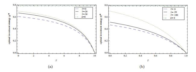
Figure 1(a) and 1(b) plot the optimal investment strategy

π^{*}

for power utility under the long and short time horizon, when the delay variable

Y

varies from

0, 20, 100

. From these figures, we conclude:

Figure 1 The effect of delay variable on the optimal strategy under power utility

Full size|PPT slide

(ⅰ) The optimal investment strategies are constant in the crash-free case, however, the optimal investment strategies are decreasing with time. The interpretation of this behaviour is obvious. With the terminal time is near, it is good to reduce investment proportion in risky asset to save the gains so as as there is not enough time to compensate the effect of a crash via an optimal stock investment afterwards.

(ⅱ) In the crash-threatened financial market, the larger is delay variable

Y

, the higher is the optimal investment proportion in risky asset. These phenomena are consistent with the practical investment behaviours. Namely, a fund manager with a good history investment performance may attract the more investment from fund investors, which encourages fund manager invest more in risky asset to achieve more performance. Contrarily, a poor history performance maybe induce investors' withdrawal, which frustrate the fund manager psychologically to draw down the proportion of wealth invested in risky asset.

(ⅲ) Figures 1(a) and 1(b) show that the optimal investment strategy is smaller in a short investment time horizon than that of in a long investment time horizon. These results can be explained by the fact that if the time horizon is short then the crash risk dominates the possibilities of obtaining a better return via stock investment, so the fund manager allocate a lower proportion in risky asset to low the risk exposure. If, however, the investment time horizon is long enough, the crash becomes a "moderate crash" which is no real threat, so the more attractive it is to invest in the stock. Nevertheless, if the final time is near then it is good to reduce stock investment as then there is not enough time to compensate the effect of a crash by means of an optimal stock investment afterwards. These result is consistent with Korn^[12].

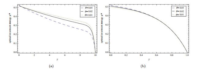
In the case of exponential utility, the optimal investment strategy does not depend on the delay variable

Y

but depend on parameter

θ

. Therefore, we plot the optimal investment strategy for exponential utility under a long and a short time horizon in Figures 2(a) and 2(b), when the parameter

θ

varies from 0.5, 0.2, 0, respectively. The two figures shows that the optimal investment strategy increases with parameter

θ

. The parameter

θ

captures the effect of delay variable

Y (T)

on the terminal fund wealth

X (T)

. That is, the larger is the parameter

θ

, the more important is the history investment performance for fund manager. Thus, the fund manager increase the proportion in risky asset with the larger

θ

. In addition, Figures 2 also shows that the optimal investment strategy is smaller in a short investment time horizon than that of in a long investment time horizon.

Figure 2 The effect of delay variable on the optimal strategy under exponential utility

Full size|PPT slide

2) The optimal strategy and crash size

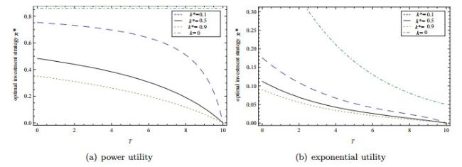
Figures 3(a) and 4(b) plot the optimal strategies

π^{*} (t)

for power utility, log utility and exponential utility, when we set different crash size

k = 0

k^{*} = 0.1

k^{*} = 0.5

and

k^{*} = 0.9

, respectively. Note that

k = 0

denote the crash-free case. The results show that the cash size has negative effect on the fund manager's investment strategy. In other words, the larger size of crash is, the less money is invested in risk asset. This makes intuitive sense. A larger crash size means higher risk and hence a fund manager invest less in risky asset under the threaten of a larger crash.

Figure 3 The effect of crash size on the optimal strategy

Full size|PPT slide

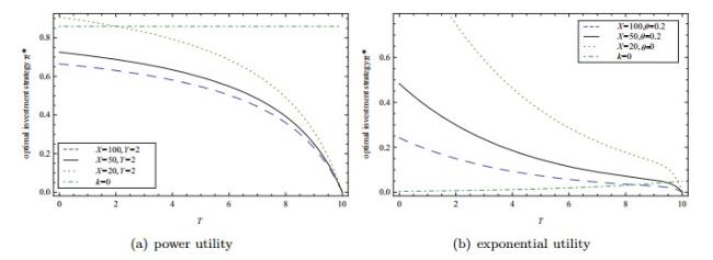
Figure 4 The effect of fund wealth level on the optimal strategy

Full size|PPT slide

From other view of bubble in financial market, a large bubble means a large threat of crash. So, in financial market where there exist large bubble, our results give a more safe and effective strategy. In other words, the investment strategy under the worst-case scenario is an equilibrium optimal strategy. If there is no crash happen at all, the worst-case model achieves a typical balance problem between obtaining good worst-case bounds for the case of a crash and also a reasonable performance. On the other hand, we can avoid greater risk if a crash does happen.

3) The optimal strategy and fund wealth level

Theorems 2 and 3 show that the optimal strategies

π^{*} (t)

are related to the fund wealth

X

. It is more reasonable that the investment strategy varies with the wealth level. Figures 4(a) and 4(b) plot the optimal strategies

π^{*} (t)

for power utility, log utility and exponential utility under the different fund wealth level:

X = 100

X = 50

X = 10

, respectively. The figures show that the optimal investment strategies

π^{*}

decrease w.r.t. wealth

X

. That is to say that the more the fund wealth does the fund manager manage, the more risk aversion the fund manager has. When a fund manager manage a larger size of fund wealth, she could bring down the proportion in the risky asset to lower her risk exposure.

6 Conclusion

In this paper, by using worst-case approach in a framework of stochastic control with delay, we have studied a portfolio optimization problem for a fund manager in a crash-threatened financial market. The financial market maybe hit crash, so it is assumed to be either in a crash-free state or in a crash state. In the crash-free state, the price of risky asset behaves as GMB and the dynamic of fund wealth is formulated as a stochastic differential delay equation. In the crash state, the price of the risky asset can suddenly drop by a certain relative amount, which leads to a dropping of the fund wealth relative to that of crash-free state. We have first formulated the worst-case portfolio optimization problem with delay and showed a verification theorem for a general utility function. Then, we have characterized the optimal strategies in general. Finally, we have derived the semi-analytical forms of optimal investment strategies and the optimal value functions in the form of ordinary differential equations for the cases of power, logarithmic, and exponential utilities. The main findings are as follows: (ⅰ) The optimal investment strategies are the function w.r.t. time and the current fund wealth. This is a difference with the result of Korn and Steffensen. In addition, the optimal investment strategies are related to the delay variable; (ⅱ) The optimal value functions are the functions w.r.t. the time, the current wealth and the delay variable; (ⅲ) The optimal investment strategies is a decreasing function w.r.t. crash size.

As illustrated in this paper, the portfolio optimization problem with a single risky and single risk-free asset obtains a semi-analytical solution. It is anticipated, however, that explicit solutions of the similar type for the model with multiple risky assets will not be available. In addition, whether it is more effective when other risk constraint such as VaR or CTE is adopted in our model. These will be a topic for future research.

References

Publishing order | Descend order by publishing year | Descend order by cited within

1	Markowitz H. Portfolio selection. Journal of Finance, 1952, 7, 77- 98. Cited in this article [1]

2	Merton R C. Lifetime portfolio selection under uncertainty: The continuous time case. Review Economic Statistics, 1969, 51 (3): 247- 257. https://doi.org/10.2307/1926560 Cited in this article [1]

3	Merton R C. Optimum consumption and portfolio rules in a continuous-time model. Journal of Economic Theory, 1971, 3 (4): 373- 413. https://doi.org/10.1016/0022-0531(71)90038-X Cited in this article [1]

4	Björk T, Murgoci A. A general theory of markovian time inconsistent stochastic control problems. Working Paper, Stockholm School of Economics, 2009. Cited in this article [1]

5	Björk T, Murgoci A. A theory of markovian time-inconsistent stochastic control in discrete time. Finance and Stochastics, 2014, 18 (3): 545- 592. https://doi.org/10.1007/s00780-014-0234-y Cited in this article [1]

6	Björk T, Murgoci A, Zhou X Y. Mean-variance portfolio optimization with state-dependent risk aversion. Mathematical Finance, 2014, 24, 1- 24. https://doi.org/10.1111/j.1467-9965.2011.00515.x Cited in this article [1]

7	Liu J, Longstaff F A, Pan J. Dynamic asset allocation with event risk. Journal of Finance, 2003, 58, 231- 259. https://doi.org/10.1111/1540-6261.00523 Cited in this article [1]

8	Cont R, Tankov P. Financial model with jump process. Chapman Hall/CRC, Printed in the United States of America, 2004. Cited in this article [1]

9	Korn R, Wilmott P. Optimal portfolios under the threat of a crash. International Journal of Theory Applied Finance, 2002, 5, 171- 187. https://doi.org/10.1142/S0219024902001407 Cited in this article [3]

10	Korn R, Menkens O. Worst-case scenario portfolio optimization: A new stochastic control approach. Mathematical Methods of Operations Research, 2005, 62, 123- 140. https://doi.org/10.1007/s00186-005-0444-3 Cited in this article [4]

11	Seifried T. Optimal investment for worst-case crash scenarios: A martingale approach. Mathematics of Operations Research, 2010, 35 (3): 559- 579. https://doi.org/10.1287/moor.1100.0459 Cited in this article [1]

12	Korn R, Steffensen M. On worst-case portfolio optimization. SIAM Journal on Control and Optimization, 2007, 46 (6): 2013- 2030. https://doi.org/10.1137/060657145 Cited in this article [9]

13	Belak C, Menkens O, Sass J. Worst-case portfolio optimization with proportional transaction costs. Working Paper, 2013. Cited in this article [1]

14	Desmettre S, Korn R, Ruckdeschel P, et al. Robust worst-case optimal investment. Working Paper, 2013. Cited in this article [1]

15	Goetzmann, William N, Ingersoll J, et al. High-water marks and hedge fund management contracts. Journal of Finance, 2003, 58, 1685- 1717. https://doi.org/10.1111/1540-6261.00581 Cited in this article [1]

16	Panageas S, Westerfield M. High-water marks: High risk appetites? Convex compensation, long horizons, and portfolio choice. Journal of Finance, 2009, 64 (1): 1- 36. https://doi.org/10.1111/j.1540-6261.2008.01427.x

17	Guasoni P, Obłój J. The incentives of hedge fund fees and high-water marks. Mathematical Finance, 2013. In press. Available at http://onlinelibrary.wiley.com/doi/10.1111/mafi.12057/pdf. Cited in this article [1]

18	Elsanosi I, Øksendal B, Sulem A. Some solvable stochastic control problems with delay. Stochastics and Stochastic Reports, 2000, 71 (1): 69- 89. Cited in this article [2]

Øksendal B, Sulem A. A maximum principle for optimal control of stochastic systems with delay, with applications to finance. Optimal Control and Partial Differential Equations-Innovations and Applications. Eds. by Menaldi J M, Rofman E, Sulem A. IOS Press, Amsterdam, The Netherlands, 2000.

Cited in this article [1]

20	Elsanousi L, Larssen B. Optimal consumption under partial observations for a stochastic system with delay. Preprint 9, University of Oslo, Oslo, Norway, 2001. Cited in this article [1]

21	Chang M H, Pang T, Yang Y P. A stochastic portfolio optimization model with bounded memory. Mathematics of Operations Research, 2011, 36 (4): 604- 619. https://doi.org/10.1287/moor.1110.0508 Cited in this article [1]

22	Federico S. A stochastic control problem with delay arising in a pension fund model. Finance and Stochastics, 2011, 15, 421- 459. https://doi.org/10.1007/s00780-010-0146-4 Cited in this article [1]

23	Shen Y, Zeng Y. Optimal investment-reinsurance with delay for mean-variance insurers: A maximum principle approach. Insurance: Mathematics and Economics, 2014, 57, 1- 12. https://doi.org/10.1016/j.insmatheco.2014.04.004 Cited in this article [1]

24	A C X, Li Z F. Optimal investment and excess-of-loss reinsurance problem with delay for an insurer under Heston's SV model. Insurance: Mathematics and Economics, 2015, 61, 181- 196. https://doi.org/10.1016/j.insmatheco.2015.01.005 Cited in this article [1]

25	Lee M K, Kim J H, Kim J. A delay financial model with stochastic volatility: Martingale method. Physica A, 2011, 390, 2909- 2919. https://doi.org/10.1016/j.physa.2011.03.032 Cited in this article [1]

26	Mao X R, Sabanis S. Delay geometric Brownian motion in financial option valuation. Stochastics: An International Journal of Probability and Stochastic Processes, 2013, 85 (2): 295- 320. https://doi.org/10.1080/17442508.2011.652965 Cited in this article [1]

27	Shen Y, Meng Q, Shi P. Maximum principle for jump-diffusion mean-field stochastic delay differential equations and its application to finance. Automatica, 2014, 50, 1565- 1579. https://doi.org/10.1016/j.automatica.2014.03.021 Cited in this article [1]

Acknowledgements

The authors gratefully acknowledge the Editor and two anonymous referees for their insightful comments and helpful suggestions that led to a marked improvement of the article.

Funding

the National Natural Science Foundation of China(71501050)

Startup Foundation for Doctors of ZhaoQing University(611-612282)

the National Science Foundation of Guangdong Province of China(2017A030310660)

PDF(355 KB)

227

Accesses

Citation

Detail

Sections

Recommended

Received	Accepted	Published
2017-01-05	2017-06-20	2018-02-25
Issue Date
2018-02-25

Please choose a citation manager

Content to export

Abstract

Key words

Cite this article

1 Introduction

2 The Model

2.1 Wealth Process

2.2 Problem Formulation

3 Verification Theorem

4 Solution

4.1 General Framework

4.2 Solution for the Power Utility

4.3 Solution for Exponential Utility

5 Numerical Simulation

Figure 1 The effect of delay variable on the optimal strategy under power utility

Figure 2 The effect of delay variable on the optimal strategy under exponential utility

Figure 3 The effect of crash size on the optimal strategy

Figure 4 The effect of fund wealth level on the optimal strategy

6 Conclusion

{{custom_sec.title}}

{{custom_sec.title}}

References

{{custom_fnGroup.title_en}}

Footnotes

Acknowledgements

{{custom_ack.title_en}}

Funding

Share

模态框（Modal）标题

Please choose a citation manager

Content to export

Abstract

Key words

Cite this article

1 Introduction

2 The Model

2.1 Wealth Process

2.2 Problem Formulation

3 Verification Theorem

4 Solution

4.1 General Framework

4.2 Solution for the Power Utility

4.3 Solution for Exponential Utility

5 Numerical Simulation

Figure 1 The effect of delay variable on the optimal strategy under power utility

Figure 2 The effect of delay variable on the optimal strategy under exponential utility

Figure 3 The effect of crash size on the optimal strategy

Figure 4 The effect of fund wealth level on the optimal strategy

6 Conclusion

{{custom_sec.title}}

{{custom_sec.title}}

References

{{custom_fnGroup.title_en}}

Footnotes

Acknowledgements

{{custom_ack.title_en}}

Funding