Optimal Insurance-Package and Investment Problem for an Insurer

Delei SHENG; Linfang XING

doi:10.21078/JSSI-2018-085-12

PDF(191 KB)

Journal of Systems Science and Information ›› 2018, Vol. 6 ›› Issue (1) : 85-96. DOI: 10.21078/JSSI-2018-085-12

Optimal Insurance-Package and Investment Problem for an Insurer

Author information +

History +

Abstract

An insurance-package is a combination being tie-in at least two different categories of insurances with different underwriting-yield-rate. In this paper, the optimal insurance-package and investment problem is investigated by maximizing the insureros exponential utility of terminal wealth to find the optimal combination-share and investment strategy. Using the methods of stochastic analysis and stochastic optimal control, the Hamilton-Jacobi-BellmanèHJBé equations are established, the optimal strategy and the value function are obtained in closed form. By comparing with classical results, it shows that the insurance-package can enhance the utility of terminal wealth, meanwhile, reduce the insureros claim risk.

Key words

insurance-package / the HJB equation / optimal combination-share / optimal strategy

Cite this article

EndNote

Ris (Procite)

Bibtex

Download Citations

Delei SHENG , Linfang XING. Optimal Insurance-Package and Investment Problem for an Insurer. Journal of Systems Science and Information, 2018, 6(1): 85-96 https://doi.org/10.21078/JSSI-2018-085-12

1 Introduction

Looking for new methods to supervise and control the risk is the important problem in current financial engineering research. For a long time, reinsurance is a widely used methods to control an insurer's claim-risk by part of its risk transferred to reinsurer. Most articles taken reinsurance into account when they studied the optimal investment problem of an insurer. For example, Irgens and Paulsen^[1] used excess of loss reinsurance and investigated the optimal control of risk exposure, reinsurance and investments for an insurance company whose insurance business follows a diffusion perturbated classical risk process. Luo, et al.^[2] considered the case of proportional reinsurance for an insurance company whose surplus is governed by a linear diffusion and given the optimal reinsurance-investment policy by minimizing the probability of ruin. Cao and Xu^[3], Gu, et al.^[4] investigated the excess-of-loss reinsurance and investment problem for an insurer's different risk process and different models of financial markets. Bai and Guo^[5] studied two optimization problems for an insurer purchasing proportional reinsurance, allowed to invest in one risk-free asset and multiple risky assets with no-shorting constraint. Also lots of recent articles, such as [6-9], studied the investment-reinsurance problem with a variety of conditions from different angle of view. The reason lies in that the reinsurance is indeed a very good tool to reduce an insurer's claim-risk. However, the disadvantage of reinsurance is obvious, because the company's risk is reduced through reinsurance, and simultaneously its potential profit reduced as well.

Just as one using portfolio — A basket of different investment assets — To reduce risk in financial market, he also can use a basket of heterogenous insurances to explore more methods of claim-risk management for an insurer. In order to reduce the risk originating in one type of insurance with high claim risk, he can put different categories of at leat two insurances into one basket and sell it as an insurance-package. An insurance-package contains no less than two different types of insurance, and the claim risk of one insurance should be significantly lower than another. In fact, people are always willing to buy the insurance products with high claim-risk but ignore those insurance products with lower claim risk. The insurance-package will substantially increase the sales volume of the insurance products with lower claim risk and provide policy holders with more comprehensive insurance services. But most of all, the insurance-package can reduce the overall claim-risk of the insurer's business.

Most of the existing literatures, the stochastic analysis of Itó and stochastic optimal control methods are mainly used. The authoritative writings about such methods, you also can refer to research papers [10-12] and etc. Based on these research methods, we focus on the optimal insurance-package and investment problem to find an optimal combination-share and an optimal investment strategy in this paper. The HJB equations are established for two different models with the goal of maximizing the expected utility of an insurer's terminal wealth, then the explicit solutions of the optimal strategies and the value functions are obtained. Theoretical analysis and some corresponding numerical examples illustrate the effects of model parameters on the optimal strategy and the optimal value function.

The rest of the paper proceeds as follows. In the next section we formulate the model. In Section 3, the insurance-package and investment problem for an insurer with two different categories of insurances is discussed and the results of a comparison situation for the classical risk model is given in Section 4. At last, some numerical examples and detailed theoretical analysis are provided in Section 5.

2 The Model

Throughout this paper,

(Ω, F, P, {F_{t}}_{0 \leq t \leq T})

denotes a complete probability space satisfying the usual condition, where

T > 0

is a finite constant representing the investment time horizon;

F_{t}

stands for the information available until time

t

. All stochastic processes introduced below are supposed to be adapted processes in this space.

The surplus process of an insurer is described by the insurance-package risk (IPR) model.

d R (t) = [(1 + θ) p_{t} λ_{1} μ_{1} + (1 + η) q_{t} λ_{2} μ_{2}] d t - d (p_{t} \sum_{i = 1}^{N_{1} (t)} X_{i} + q_{t} \sum_{j = 1}^{N_{2} (t)} Y_{j}) .

(1)

An insurance-package is determined by the combination-share

(p_{t}, q_{t})

of two different categories of insurance.

\sum_{i = 1}^{N_{1} (t)} X_{i}, \sum_{j = 1}^{N_{2} (t)} Y_{j}

represent the cumulative claims until time

t

for two different types of insurance, insurance 1 and insurance 2, respectively.

N_{1} (t), N_{2} (t)

are two homogeneous Poisson process with intensity

λ_{1}, λ_{2}

and the claim sizes

{X_{i}, i \geq 1}, {Y_{j}, j \geq 1}

are independent random variables.

E [X_{i}] = μ_{1}

and

E [X_{i}^{2}] = σ_{1}^{2}

E [Y_{j}] = μ_{2}

and

E [Y_{j}^{2}] = σ_{2}^{2}

. The premium according to the expected value principle, where

η > θ > 0

denotes the safety loading of two different categories of insurance, which means that the claim risk of insurance 1 is higher than insurance 2.

The risk process of the insurer can be approximated by a diffusion process according to Grandell^[10] in the following form

d R (t) = (θ p_{t} λ_{1} μ_{1} + η q_{t} λ_{2} μ_{2}) d t + \sqrt{λ_{1} σ_{1}^{2} p_{t}^{2} + λ_{2} σ_{2}^{2} q_{t}^{2}} d W (t) .

Moreover, the insurer also can invest in a financial market consisting of one risk-free asset and one risky asset. The price process

S_{0} (t)

of the risk-free asset is given by

d S_{0} (t) = r S_{0} (t) d t,

where

r > 0

is the risk-free interest rate.

The price process

S (t)

of the risky asset is described by

d S (t) = S (t) [α d t + β d \hat{W} (t)],

(2)

where

α, β

are positive constants,

α > r

is the expected instantaneous return rate of the risky asset;

\hat{W} (t)

is a standard Brownian motion. In this paper, we assume the standard Brownian motions

\hat{W} (t)

is independent with

W (t)

The control

Λ = {(p_{t}, q_{t}, π_{t}) : t \in [0, T]}

, and

π_{t}

represents the amount invested in the risky asset. Here, short-selling is not allowed, i.e.,

π_{t} \geq 0

. The amount invested in the risk-free asset is

X (t) - π_{t}

, where

X (t)

is the wealth process for the insurer under the strategy

Λ

The corresponding reserve process is given by the following dynamics of

X (t)

{\begin{cases} d X (t) = & [θ p_{t} λ_{1} μ_{1} + η q_{t} λ_{2} μ_{2} + r X (t) + (α - r) π_{t}] d t \\ + β π_{t} d \hat{W} (t) + \sqrt{λ_{1} σ_{1}^{2} p_{t}^{2} + λ_{2} σ_{2}^{2} q_{t}^{2}} d W (t), \\ X (0) = & x_{0} . \end{cases}

(3)

A strategy

Λ = (p_{t}, q_{t}, π_{t})

is said to be admissible, if

\forall t \in [0, T]

(p_{t}, q_{t}, π (t))

F (t)

progressively measurable,

E [\int_{0}^{\infty} π_{t}^{2} d t < \infty]

and (3) has a unique (strong) solution. Denote by

Ξ

the set of all admissible strategies. Suppose the insurer aims to maximize the expected utility of his/her terminal wealth and has a utility function

U (x)

which is strictly concave and continuously differentiable on

(- \infty, + \infty)

, i.e.,

max_{Λ \in Ξ} E [U (X (T))] .

(4)

For an admissible strategy

Λ = (p_{t}, q_{t}, π_{t})

, we define the value function as

H^{Λ} (t, x) = E [U (X (T)) | X (t) = x]

and the optimal value function is

H (t, x) = sup_{Λ \in Ξ} H^{Λ} (t, x), H (T, x) = U (x) .

The objective of the insurer is to find an optimal strategy

Λ^{*} = (p^{*}, q^{*}, π^{*})

such that

H (t, x) = H^{Λ^{*}} (t, x),

(5)

where

H (t, x)

is the optimal value function and

π^{*}

is the optimal investment strategy.

3 Main Results

In this section, we consider the solution of the insurance-package and investment problem to maximize the expected utility of terminal wealth, and the insurer has an common exponential utility function

U (x) = u_{0} - \frac{1}{b} e^{- b x}, b > 0.

This utility function has a constant absolute risk aversion parameter

b

, and is the only utility function under the principle of "zero utility" giving a fair premium that is independent of the level of reserves of insurers.

Theorem 1 For the insurance-package and investment problem, suppose all assumptions of this paper holds. The optimal value function is

V (t, x) = u_{0} - \frac{1}{b} \exp {- b x e^{- r (t - T)} + (\frac{λ_{1} θ^{2} μ_{1}^{2}}{2 σ_{1}^{2}} + \frac{λ_{2} η^{2} μ_{2}^{2}}{2 σ_{2}^{2}} + \frac{(α - r)^{2}}{2 β^{2}}) (t - T)}, b > 0,

and the optimal strategy is given by $Λ^{*} = (p^{*}, q^{*}, π^{*})$ , where

p^{*} = \frac{θ μ_{1}}{b σ_{1}^{2}} e^{r (t - T)}, q^{*} = \frac{η μ_{2}}{b σ_{2}^{2}} e^{r (t - T)},

and

π^{*} = \frac{(α - r)}{b β^{2}} e^{r (t - T)} .

Proof. Applying the classical tools of stochastic optimal control, if the optimal value function

H (t, x) \in C^{1, 2} ([0, T] \times R)

, then

H

satisfies the following Hamilton-Jacobi-Bellman (HJB) equation:

\begin{array}{ll} H_{t} + r x H_{x} + max_{p} {θ p λ_{1} μ_{1} H_{x} + \frac{1}{2} λ_{1} σ_{1}^{2} p^{2} H_{x x}} \\ + max_{q} {η q λ_{2} μ_{2} H_{x} + \frac{1}{2} λ_{2} σ_{2}^{2} q^{2} H_{x x}} + max_{π} {(α - r) π H_{x} + \frac{1}{2} β^{2} π^{2} H_{x x}} = 0, \end{array}

(6)

where

H_{t}, H_{x}, H_{x x}

denote the corresponding first and second-order partial derivatives of

H (t, x)

with respect to (w.r.t.) the corresponding variables, respectively.

Taking the derivative of (6) with respect to

p, q, π

, respectively. According to the first-order necessary condition, the optimal strategy

(p^{*}, q^{*}, π^{*})

is given by

{\begin{cases} p^{*} & = - \frac{θ μ_{1}}{σ_{1}^{2}} \frac{H_{x}}{H_{x x}}, \\ q^{*} & = - \frac{η μ_{2}}{σ_{2}^{2}} \frac{H_{x}}{H_{x x}}, \\ π^{*} & = - \frac{(α - r)}{β^{2}} \frac{H_{x}}{H_{x x}} . \end{cases}

(7)

Putting (7) into (6), after a simple calculation, get the result

H_{t} + r x H_{x} - \frac{λ_{1} θ^{2} μ_{1}^{2}}{2 σ_{1}^{2}} \frac{H_{x}^{2}}{H_{x x}} - \frac{λ_{2} η^{2} μ_{2}^{2}}{2 σ_{2}^{2}} \frac{H_{x}^{2}}{H_{x x}} - \frac{(α - r)^{2}}{2 β^{2}} \frac{H_{x}^{2}}{H_{x x}} = 0.

(8)

To solve this equation, we try to conjecture a solution

V (t, x)

in the following way:

V (t, x) = u_{0} - \frac{1}{b} \exp {- b x f (t) + g (t)}, b > 0, f (T) = 1, g [T] = 0 .

For this conjecture, take the first-order/second-order partial derivatives of it with respect to

t, x

V_{t} = V [- b x f^{'} (t) + g^{'} (t)], V_{x} = V [- b f (t)], V_{x x} = V b^{2} f (t)^{2} .

Substituting the above derivatives into (8), it yields

- b x f^{'} (t) + g^{'} (t) - r x b f (t) - \frac{λ_{1} θ^{2} μ_{1}^{2}}{2 σ_{1}^{2}} - \frac{λ_{2} η^{2} μ_{2}^{2}}{2 σ_{2}^{2}} - \frac{(α - r)^{2}}{2 β^{2}} = 0.

Split it into the following two equations

{\begin{cases} - b x f^{'} (t) - r x b f (t) = 0, \\ g^{'} (t) - \frac{λ_{1} θ^{2} μ_{1}^{2}}{2 σ_{1}^{2}} - \frac{λ_{2} η^{2} μ_{2}^{2}}{2 σ_{2}^{2}} - \frac{(α - r)^{2}}{2 β^{2}} = 0. \end{cases}

To solve the two ordinary differential equations with

f (T) = 1, g (T) = 0

, you can obtain the accurate solutions

f (t) = e^{- r (t - T)}

and

g (t) = (\frac{λ_{1} θ^{2} μ_{1}^{2}}{2 σ_{1}^{2}} + \frac{λ_{2} η^{2} μ_{2}^{2}}{2 σ_{2}^{2}} + \frac{(α - r)^{2}}{2 β^{2}}) (t - T) .

The optimal value function is

V (t, x) = u_{0} - \frac{1}{b} \exp {- b x e^{- r (t - T)} + (\frac{λ_{1} θ^{2} μ_{1}^{2}}{2 σ_{1}^{2}} + \frac{λ_{2} η^{2} μ_{2}^{2}}{2 σ_{2}^{2}} + \frac{(α - r)^{2}}{2 β^{2}}) (t - T)}, b > 0,

(9)

and the optimal strategy

Λ^{*} = (p^{*}, q^{*}, π^{*})

is given by

p^{*} = \frac{θ μ_{1}}{b σ_{1}^{2}} e^{r (t - T)}, q^{*} = \frac{η μ_{2}}{b σ_{2}^{2}} e^{r (t - T)}, π^{*} = \frac{(α - r)}{b β^{2}} e^{r (t - T)} .

Remark 1 The results obtained here are crisp and clear. The combination-share of the insurance with higher claim-risk is

p^{*} = \frac{θ μ_{1}}{b σ_{1}^{2}} e^{r (t - T)} = \frac{1}{b} \cdot \frac{θ μ_{1}}{σ_{1}^{2}} \cdot e^{r (t - T)},

the combination-share of the insurance with lower claim-risk is

q^{*} = \frac{η μ_{2}}{b σ_{2}^{2}} e^{r (t - T)} = \frac{1}{b} \cdot \frac{η μ_{2}}{σ_{2}^{2}} \cdot e^{r (t - T)}

and the optimal investment amount on the risk asset is

π^{*} = \frac{(α - r)}{b β^{2}} e^{r (t - T)} = \frac{1}{b} \cdot \frac{(α - r)}{β^{2}} \cdot e^{r (t - T)} .

It's easy to see that

e^{r (t - T)}

is a discount factor with the interest rate

r

and

\frac{1}{b}

reveals the influence of an insurer's absolute risk aversion coefficient on their decisions. As for

\frac{θ μ_{1}}{σ_{1}^{2}}

\frac{η μ_{2}}{σ_{2}^{2}}

and

\frac{(α - r)}{β^{2}}

, they are relative ratios of returns on risk-taking. So the economic meanings of them are obvious.

Similar to Fleming and Soner^[11], we can give a verification theorem and the proof as follows.

Theorem 2 (verification theorem) Let $V (t, x)$ be a convex, twice differential solution to $(8)$ with the boundary condition $V (T, x) = U (x)$ such that $| V (0, x_{0}) | < \infty$ . Then, for all $t \in [0, T], x \in (0, \infty)$ :

$(I)$ $V (t, x) \leq H^{Λ} (t, x)$ for every admissible strategy $Λ \in Ξ$ .

$(I I)$ If there exists an admissible control $Λ^{*} = (p^{*}, q^{*}, π^{*})$ such that

Λ^{*} \in \arg max [A^{Λ} H (t, x^{*} (t))],

where

A^{Λ} V (t, x) = V_{t} + V_{x} [θ p_{t} λ_{1} μ_{1} + η q_{t} λ_{2} μ_{2} + r x + (α - r) π_{t}] + \frac{1}{2} [β^{2} π_{t}^{2} + λ_{1} σ_{1}^{2} p_{t}^{2} + λ_{2} σ_{2}^{2} q_{t}^{2}] V_{x x} .

Then the value function $H (t, x) = H^{Λ^{*}} (t, x) = V (t, x)$ and the policy $Λ^{*} = (p^{*}, q^{*}, π^{*})$ is the optimal strategy corresponding to $X^{Λ^{*}} (t)$ which is the solution of $(3)$ .

Proof. The proof is classical, omitted here.

4 The Results of Classical Model

The surplus process of an insurer is described by the classical risk model.

d R (t) = [(1 + θ) λ_{1} μ_{1}] d t - d (\sum_{i = 1}^{N_{1} (t)} X_{i}),

(10)

where

\sum_{i = 1}^{N_{1} (t)} X_{i}

represents the cumulative claims until time

t

, where

N_{1} (t)

is a homogeneous Poisson process with intensity

λ_{1}

and the claim sizes

{X_{i}, i \geq 1}

are independent random variables. Denote the mean value

E [X_{i}] = μ_{1}

and

E [X_{i}^{2}] = σ_{1}^{2}

. The premium according to the expected value principle, where

η > 0

denotes the safety loading, which means that the claim risk of insurance 1.

The continuous form of an insurer's risk process can be approximated by a diffusion process according to Grandell[10], given by

d R (t) = θ λ_{1} μ_{1} d t + \sqrt{λ_{1}} σ_{1} d W (t) .

Moreover, the insurer also can invest in a financial market consisting of one risk-free asset and one risky asset. The price process

S_{0} (t)

of the risk-free asset is given by

d S_{0} (t) = r S_{0} (t) d t,

where

r > 0

is the risk-free interest rate.

The price process

S (t)

of the risky asset is described by

d S (t) = S (t) (α d t + β d \hat{W} (t)),

(11)

where

α, β

are positive constants,

α > r

is the expected instantaneous return rate of the risky asset;

\hat{W} (t)

is a standard Brownian motion. In this paper, we assume the standard Brownian motions

\hat{W} (t)

is independent with

W (t)

The control

Π = {π_{t} | t \in [0, T]}

, and

π_{t}

represents the amount invested in the risky asset. Here, short-selling is not allowed, i.e.,

π_{t} \geq 0

. The amount invested in the risk-free asset is

X (t) - π_{t}

, where

X (t)

is the wealth process for the insurer under the strategy

π

and the dynamics of

X (t)

is given by

{\begin{cases} d X (t) = [θ λ_{1} μ_{1} + r X (t) + (α - r) π_{t}] d t + β π d \hat{W} (t) + \sqrt{λ_{1}} σ_{1} d W (t), \\ X (0) = x_{0} . \end{cases}

(12)

A strategy

π_{t}

is said to be admissible, if

\forall t \in [0, T]

π (t)

F (t)

progressively measurable,

E [\int_{0}^{\infty} π_{t}^{2} d t < \infty]

and (12) has a unique (strong) solution. Denote by

Π

the set of all admissible strategies. Suppose the insurer aims to maximize the expected utility of his/her terminal wealth and has a utility function

U (x)

which is strictly concave and continuously differentiable on

(- \infty, + \infty)

, i.e.,

max_{π \in Π} E [U (X (T))] .

(13)

In the rest of this section, we consider the solution of classical investment problem to maximize the expected utility of terminal wealth, and the insurer has an common exponential utility function

U (x) = u_{0} - \frac{1}{b} e^{- b x}, b > 0

, which has a constant absolute risk aversion parameter

b

. For an admissible strategy

π_{t}

, we define the value function as

H^{π} (t, x) = E [U (X (T)) | X (t) = x]

and the optimal value function is

H (t, x) = sup_{π \in Π} H^{π} (t, x), H (T, x) = U (x) .

The objective of the insurer is to find an optimal strategy

π^{*}

such that

H (t, x) = H^{π^{*}} (t, x)

, where

H (t, x)

is the optimal value function and

π^{*}

is the optimal investment strategy.

Theorem 3 For the optimal investment problem under the classical risk model, suppose all assumptions of this paper holds. The optimal investment strategy is given by

π^{*} = \frac{(α - r)}{b β^{2}} e^{r (t - T)},

and the optimal value function is

V (t, x) = u_{0} - \frac{1}{b} \exp {- b x e^{- r (t - T)} + g (t)}, b > 0,

where

g (t) = \frac{e^{- 2 r t} (- 4 b e^{r (t + T)} β^{2} θ λ_{1} μ_{1} + b^{2} e^{2 r T} β^{2} λ_{1} σ_{1}^{2}) + (2 r (t - T) (r - α)^{2} + b β^{2} λ_{1} (4 θ μ_{1} - b σ_{1}^{2}))}{4 r β^{2}} .

Proof. Applying the classical tools of stochastic optimal control, if the optimal value function

H (t, x) \in C^{1, 2} ([0, T] \times R)

, then

H

satisfies the following Hamilton-Jacobi-Bellman (HJB) equation:

H_{t} + (r x + θ λ_{1} μ_{1}) H_{x} + \frac{1}{2} λ_{1} σ_{1}^{2} H_{x x} + max_{π} {(α - r) π H_{x} + \frac{1}{2} β^{2} π^{2} H_{x x}} = 0,

(14)

where

H_{t}, H_{x}, H_{x x}

denote the corresponding first and second-order partial derivatives of

H (t, x)

with respect to (w.r.t.) the corresponding variables, respectively. Taking the derivative of the left of this HJB equation with respect to

π

. According to the first-order necessary condition, the optimal strategy

π

is given by

π^{*} = - \frac{(α - r)}{β^{2}} \frac{H_{x}}{H_{x x}} .

Putting

π^{*}

into (14), after a simple calculation, get the result

H_{t} + (r x + θ λ_{1} μ_{1}) H_{x} + \frac{1}{2} λ_{1} σ_{1}^{2} H_{x x} - \frac{(α - r)^{2}}{2 β^{2}} \frac{H_{x}^{2}}{H_{x x}} = 0.

(15)

To solve this equation, we try to conjecture a solution

V (t, x)

in the following way:

V (t, x) = u_{0} - \frac{1}{b} \exp {- b x f (t) + g (t)}, b > 0, f (T) = 1, g (T) = 0 .

For this conjecture, take the first-order/second-order partial derivatives of it with respect to

t

x

V_{t} = V [- b x f^{'} (t) + g^{'} (t)], V_{x} = V [- b f (t)], V_{x x} = V b^{2} f (t)^{2} .

Substituting the above derivatives into (15), it yields

V [- b x f^{'} (t) + g^{'} (t)] + (r x + θ λ_{1} μ_{1}) V [- b f (t)] + \frac{1}{2} λ_{1} σ_{1}^{2} V b^{2} f (t)^{2} - \frac{(α - r)^{2}}{2 β^{2}} \frac{(V [- b f (t)])^{2}}{V b^{2} f (t)^{2}} = 0.

After the simplification,

- b x f^{'} (t) + g^{'} (t) - (r x + θ λ_{1} μ_{1}) b f (t) + \frac{1}{2} λ_{1} σ_{1}^{2} b^{2} f (t)^{2} - \frac{(α - r)^{2}}{2 β^{2}} = 0 .

Split the above equation into the following two equations

{\begin{cases} - b x f^{'} (t) - r x b f (t) = 0, \\ g^{'} (t) - θ λ_{1} μ_{1} b f (t) + \frac{1}{2} λ_{1} σ_{1}^{2} b^{2} f (t)^{2} - \frac{(α - r)^{2}}{2 β^{2}} = 0. \end{cases}

To solve the two ordinary differential equations with

f (T) = 1, g (T) = 0

, you can obtain the accurate solutions

f (t) = e^{- r (t - T)}

and

g (t) = \frac{e^{- 2 r t} (- 4 b e^{r (t + T)} β^{2} θ λ_{1} μ_{1} + b^{2} e^{2 r T} β^{2} λ_{1} σ_{1}^{2}) + (2 r (t - T) (r - α)^{2} + b β^{2} λ_{1} (4 θ μ_{1} - b σ_{1}^{2}))}{4 r β^{2}} .

The optimal value function is

V (t, x) = u_{0} - \frac{1}{b} \exp {- b x e^{- r (t - T)} + g (t)}, b > 0,

and the optimal strategy is given by

π^{*} = \frac{(α - r)}{b β^{2}} e^{r (t - T)} .

5 Numerical Results

In this section, some numerical analysis and graphics are provided to illustrate our results. Unless otherwise stated, the hypothetical values of model parameters are as follows.

Table 1 Numerical values of model parameters

$θ$	$η$	$λ_{1}$	$μ_{1}$	$b$	$β$	$u_{0}$	$r$	$T$	$α$	$σ_{1}$	$λ_{2}$	$μ_{2}$	$σ_{2}$
0.1	0.06	1	0.2	1	2	5	0.015	5	0.15	1	1	0.1	0.6

In the following, the analysis of the two value functions are compared to see the utility differences. The optimal value function of the insurance-package and investment problem

V (t, x) = u_{0} - \frac{1}{b} \exp {- b x e^{- r (t - T)} + (\frac{λ_{1} θ^{2} μ_{1}^{2}}{2 σ_{1}^{2}} + \frac{λ_{2} η^{2} μ_{2}^{2}}{2 σ_{2}^{2}} + \frac{(α - r)^{2}}{2 β^{2}}) (t - T)}, b > 0,

and the optimal value function of the classical risk model

V (t, x) = u_{0} - \frac{1}{b} \exp {- b x e^{- r (t - T)} + g (t)}, b > 0,

where

g (t) = \frac{e^{- 2 r t} (- 4 b e^{r (t + T)} β^{2} θ λ_{1} μ_{1} + b^{2} e^{2 r T} β^{2} λ_{1} σ_{1}^{2}) + (2 r (t - T) (r - α)^{2} + b β^{2} λ_{1} (4 θ μ_{1} - b σ_{1}^{2}))}{4 r β^{2}} .

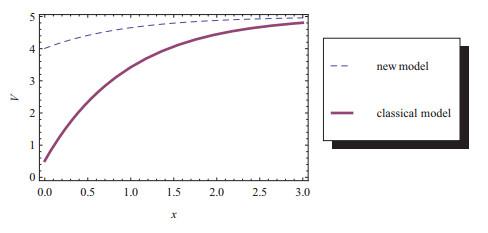
Using an insurance-package, the insurer's utility of terminal wealth is enhanced significantly. Figure 1 shows that the utility is always increases with wealth amount and the utility of the new operation mode using insurance-package can create greater utility of terminal wealth for insurers.

Figure 1 The utility functions

Full size|PPT slide

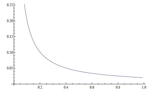
It is noteworthy that the capital amount invested in risk assets has nothing to do with the total amount of wealth, but only depends on the risk premium, the risk aversion degree of the insurer and the volatility of risk asset.

π^{*} = \frac{1}{b} \frac{(α - r)}{β^{2}} e^{r (t - T)} .

The impact of an insurer's risk aversion degree on investment decision-making is very obvious. Figure 2 shows that the investment amount on risk asset significantly decrease with the increasing of an insurer's risk aversion degree.

Figure 2 The investment strategy of different risk aversion

Full size|PPT slide

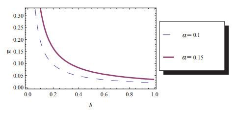
Whatever your degree of risk aversion, the higher rate of investment return is always has a strong appeal to investors. Figure 3 shows that the higher yield of the risk asset investment always win larger volume of investment for investors with different levels of risk aversion.

p^{*} = \frac{θ μ_{1}}{b σ_{1}^{2}} e^{r (t - T)}, q^{*} = \frac{η μ_{2}}{b σ_{2}^{2}} e^{r (t - T)} .

Figure 3 The investment strategy of different rate of return

Full size|PPT slide

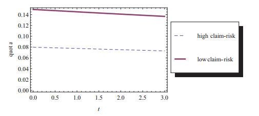
The optimal combination-share of selected insurance can give a similar interpretation, if

σ_{1}^{2}, σ_{2}^{2}

being considered as the claim-risk measure of two different insurances and

θ μ_{1}, η μ_{2}

representing the corresponding revenue compensation of claim risk, respectively. The revenue compensation of claim risk divided by the claim risk measurement can give us a ratio. The ratio is a very important indicator, which directly decided the combination-share of a specific insurance in an insurance-package, for convenience, it's referred to as underwriting-yield-rate in this paper. Figure 4 shows us that a specific insurance with higher underwriting-yield-rate must lead to higher combination-share of this insurance in an insurance-package.

Figure 4 The quota of different categories of insurance

Full size|PPT slide

6 Conclusion

In this paper, we generalize the classical risk model with an insurance-package of at least two different kinds of insurance to describe an insurer risk process. With the dynamics of risky assets' prices described by the geometric Brownian motion, the optimal insurance-package and investment problem is investigated by maximizing the insurer's exponential utility of terminal wealth. Hamilton-Jacobi-Bellman (HJB) equations are established and the explicit solution are obtained. The amazing discovery is that the amount of risk asset investment has nothing to do with insurer's wealth and it's insurance business, which is consistent with previous research conclusion. Comparing with the results of classical model, we also found that underwriting-yield-rate — Revenue compensation of claim risk divided by the claim risk measurement — Is the key factor to decide the combination-share of a specific insurance in an insurance-package.

References

Publishing order | Descend order by publishing year | Descend order by cited within

1	Irgens C, Paulsen J. Optimal control of risk exposure, reinsurance and investments for insurance portfolios. Insurance Mathematics and Economics, 2004, 35 (1): 21- 51. https://doi.org/10.1016/j.insmatheco.2004.04.004 Cited in this article [1]

2	Luo S, Taksar M, Tsoi A. On reinsurance and investment for large insurance portfolios. Insurance Mathematics and Economics, 2008, 42 (1): 434- 444. https://doi.org/10.1016/j.insmatheco.2007.04.002 Cited in this article [1]

3	Cao Y, Xu J. Proportional and excess-of-loss reinsurance under investment gains. Applied Mathematics and Computation, 2010, 217 (6): 2546- 2550. https://doi.org/10.1016/j.amc.2010.07.067 Cited in this article [1]

4	Gu A, Guo X, Li Z, et al. Optimal control of excess-of-loss reinsurance and investment for insurers under a CEV model. Insurance: Mathematics and Economics, 2012, 51 (3): 674- 684. https://doi.org/10.1016/j.insmatheco.2012.09.003 Cited in this article [1]

5	Bai L, Guo J. Optimal proportional reinsurance and investment with multiple risky assets and no-shorting constraint. Insurance Mathematics and Economics, 2008, 42 (3): 968- 975. https://doi.org/10.1016/j.insmatheco.2007.11.002 Cited in this article [1]

6	Zhao H, Shen Y, Zeng Y. Time-consistent investment-reinsurance strategy for mean-variance insurers with a defaultable security. J. Math. Anal. Appl., 2016, 437 (2): 1036- 1057. https://doi.org/10.1016/j.jmaa.2016.01.035 Cited in this article [1]

7	Yao D, Yang H, Wang R. Optimal dividend and reinsurance strategies with financing and liquidation value. Astin Bulletin, 2016, 1 (2): 1- 35.

8	Huang Y, Yang X, Zhou J. Optimal investment and proportional reinsurance for a jump-diffusion risk model with constrained control variables. Journal of Computational and Applied Mathematics, 2016, 296 (C): 443- 461.

9	Sheng D L. Explicit solution of reinsurance-investment problem for an insurer with dynamic income under vasicek model. Advances in Mathematical Physics, 2016, 2016 (1): 1- 13. Cited in this article [1]

10	Grandell J. Aspects of risk theory. Springer-Verlag, 1991. Cited in this article [3]

11	Fleming H U, Soner H M. Controlled Markov processes and viscosity solutions. Springer, 1993. Cited in this article [1]

12	Browne S. Optimal investment policies for a firm with a random risk process: Exponential utility and minimizing the probability of ruin. Mathematics of Operations Research, 1995, 20 (4): 937- 958. https://doi.org/10.1287/moor.20.4.937 Cited in this article [1]

Acknowledgements

This research was supported by China Postdoctoral Science Foundation Funded Project (2017M611192) and also supported by Youth Science Fund of Shanxi University of Finance and Economics (QN-2017019).

Funding

Youth Science Fund of Shanxi University of Finance and Economics(QN-2017019)

PDF(191 KB)

216

Accesses

Citation

Detail

Sections

Recommended

Abstract
Key words
Cite this article
1 Introduction
2 The Model
3 Main Results
4 The Results of Classical Model
5 Numerical Results
Table 1 Numerical values of model parameters
Figure 1 The utility functions
Figure 2 The investment strategy of different risk aversion
Figure 3 The investment strategy of different rate of return
Figure 4 The quota of different categories of insurance
6 Conclusion
References
Acknowledgements
Funding

Received	Accepted	Published
2016-12-09	2017-03-09	2018-02-25
Issue Date
2018-02-25

Please choose a citation manager

Content to export

Abstract

Key words

Cite this article

1 Introduction

2 The Model

3 Main Results

4 The Results of Classical Model

5 Numerical Results

Table 1 Numerical values of model parameters

Figure 1 The utility functions

Figure 2 The investment strategy of different risk aversion

Figure 3 The investment strategy of different rate of return

Figure 4 The quota of different categories of insurance

6 Conclusion

{{custom_sec.title}}

{{custom_sec.title}}

References

{{custom_fnGroup.title_en}}

Footnotes

Acknowledgements

{{custom_ack.title_en}}

Funding

Share

模态框（Modal）标题

Please choose a citation manager

Content to export

Abstract

Key words

Cite this article

1 Introduction

2 The Model

3 Main Results

4 The Results of Classical Model

5 Numerical Results

Table 1 Numerical values of model parameters

Figure 1 The utility functions

Figure 2 The investment strategy of different risk aversion

Figure 3 The investment strategy of different rate of return

Figure 4 The quota of different categories of insurance

6 Conclusion

{{custom_sec.title}}

{{custom_sec.title}}

References

{{custom_fnGroup.title_en}}

Footnotes

Acknowledgements

{{custom_ack.title_en}}

Funding