1 Introduction
The fast development of the electronic trading system in many established exchanges leads to the sharp decrease of the order processing time during stock trading. As a result, high-frequency trading (HFT), which executes orders within minutes or seconds, proliferated and has accounted for more than 50% of stock trades in the US and Europe. Recently, HFT started to rise in Asian markets.
HFT relies on high-frequency stock price prediction, while the high nonlinearity and time variability of stock price make the prediction very challenging. Traditional prediction methods such as statistical modeling typically impose strict but unvalidated mathematical assumptions on data, which are difficult to apply in the real world
[1-3]. Recent literature has demonstrated a great interest in using machine learning techniques in this area owing to their data-driven characteristic and light-weight computation
[4-10].
Technical indicators are often used as inputs for high-frequency stock trend prediction using machine learners. One of the critical issues is how to determine the set of informative and discriminating input indicators. Good prediction naturally requires as much as inputs, but too many of them will result in the problem of "curse of dimensionality". Some technical indicators are considered to have good discriminating capacity in the literature. A typical input set includes the moving average (MA), exponential moving average (EMA), relative strength index (RSI), relative difference price (RDP), moving average convergence and divergence (MACD), and possibly other metrics
[11-16]. However, most of the current studies aim to predict daily stock price, in which these indicators are often set over a certain number of days according to experts' experience. For example, MA and RDP are commonly used with a period parameter of 5- or 10-days, RSI with 6- or 12-days and MACD with 12- or 26-days
[16, 17]. Until now, there is no gold standard to determine the proper set of technical indicators and their period parameters for high-frequency stock prediction.
To circumvent this issue, we propose to use an adaptive input selection (AIS) approach to select the most suitable indicators and their period parameters for the high-frequency stock trend prediction using machine learners. This approach is implemented by incorporating a feature selection technique, such as $ t $-statistics, information gain, ROC or PCA methods, into the prediction procedure. In the end, we compute the performance of the AIS approach for the 5-minute ahead prediction of CSI 300 index and compared it with the commonly used deterministic input setting (DIS) approach. The experiment is based on two state-of-the-art learners that has shown excellent performance in stock prediction: Support vector machines (SVM) and artificial neural networks (ANN).
This paper is organized as follows: Section 2 provides a brief background of feature selection techniques, machine learning algorithms and prediction performance evaluation criteria. Section 3 describes the research data and experimental procedures. Section 4 shows and discusses the results. Section 5 concludes the study.
2 Backgrouds
2.1 Feature Selection Techniques
Given training data $ D = \{(x_i, y_i), i = 1, 2, \cdots, n\} $, where every vector $ x_i $ has $ d $ features and $ y_i\in\{1, 0\} $ denotes that each $ x_i $ belongs to class 1 or 0. The number of instances belonging to class 1 or 0 is $ n_1 $ and $ n_0 $.
2.1.1 T-Statistics
An independent $ t $-statistics is often used to rank and select features. For a given feature $ A $ of $ x $, the mean $ \mu_1 $ (resp. $ \mu_0 $) and the standard deviation $ s_1 $ (resp. $ s_0 $) of the samples belonging to class 1 (resp. 0) are calculated. Then the $ t $-statistics on $ A $ is defined by
$ T(A) = \frac{|\mu_1- \mu_0|}{\sqrt{\frac{(s_1)^2}{n_1}+\frac{(s_0)^2}{n_0}}}, $ where $ n_1 $ and $ n_0 $ are the number of samples in class 1 and 0 respectively.
2.1.2 Information Gain
Information gain reflects the additional information about a class provided by a given feature. For the feature $ A $, its information gain is defined by
$ \begin{align*} IG(A) = \sum\limits_{x_i}p(x_i)\sum\limits_{y_i}p(y_i|x_i(A))\log_2p(y_i|x_i(A)) - \sum\limits_{y_i}p(y_i)\log_2p(y_i), \end{align*} $ where $ x_i(A) $ denotes the value of feature $ A $ in $ x_i $.
2.1.3 Receiver Operating Characteristic
The receiver operating characteristic (ROC) curve describes the performance of a binary classifier system as the threshold on a feature varies, thus provides a tool to measure the discriminating power of a given feature. It plots the true positive rate against the false positive rate at various threshold settings. Feature rank by ROC method computes the area under the ROC curve, which is defined as the probability that a randomly chosen instance of class 1 ranks higher than that of class 0.
2.1.4 Principle Component Analysis
Principle component analysis (PCA) is a method that transforms the data into a new space but retains most of the variation. It first computes the covariance matrix of the original features and then extracts the eigenvectors of the matrix. These eigenvectors define an orthogonal linear transformation that maps the original feature space to a new one where the features are uncorrelated. Each eigenvector constructs a new feature vector and its corresponding eigenvalue gives the significance of the new feature.
2.2 Machine Learning Techniques
2.2.1 Support Vector Machine
For the dataset $ D $, a classical support vector machine (SVM) learns to find the function of a hyperplane
$ \begin{equation} f(x) = k(w, x)+b, \end{equation} $
that classifies the observations into class 1 or class 0. $ k(x_i, x_j) $ is a kernel function that maps the input feature vector $ x_i\in R^d $ in to a higher dimension space. There are many types of kernel functions for SVM, and in our study, the state-of-art radial basis kernel function is used. The solution of $ w $ can be found by maximizing the distance between the hyperplane and the nearest sample point of the two classes $ 2/\|w\|^2 $ as well as minimizing the misclassification error. The dual form of the Lagrangian function of the optimization problem can be written as
$ \begin{equation} L_D = \sum\limits_{i=1}^n \alpha_i - \frac{1}{2} \alpha_i\alpha_jy_iy_jk(x_i, x_j), \end{equation} $
subjected to the constraints $ 0\leq \alpha_i \leq c $ and $ \sum_{i=1}^n \alpha_iy_i = 0 $. Here, the regularization parameter $ c $ controls the trade-off between the margin and the misclassification error. $ w $ is then given by
$ w = \sum\limits_i \alpha^*_iy_ik(x_i, \cdot), $ where $ \alpha^*_i $ is the solution of Equation (2).
After an SVM classifier is obtained, a new instance is classified into class 1 if $ f(x)>0 $ and into class 0 otherwise.
2.2.2 Artificial Neural Network
By mimicking a biological brain, artificial neural networks (ANN) construct a dense network with inner-connected neurons. Each of the neurons in the network gets activated by several inputs and gives one output value. The output value is computed through an activation function, which can be the linear function, sigmoid function or tanh function. A typical network usually consists one input layer, several hidden layers and one output layer. The input layer has several neurons, each of which receives one value from one input feature and compute one output value. Each of the hidden layers combines the output values of the previous layer as input values to each hidden neurons, and the combinations are different from one neuron to another regarding the combination weights. The optimal weights are pursued through learning on the training set. The output layer takes all the output values of the last hidden layer to compute a final output value.
In this study, we use a three layer feed-forward neural network, in which tan sigmoid is used as the activation function for all layers. Gradient descent method with momentum is used to compute the optimal weights at each epoch and the number of epochs is fixed to 1000. The value of learning rate in the minimization process with gradient descent method is set to 0.1. The momentum $ mc $ in the minimization process and the number of neurons $ n $ in the hidden layer are parameters to be set through learning on the training set. A threshold of 0.5 for the final output value is used to determine the prediction class of an instance. Namely, if the output value is greater than 0.5, the instance is considered to be in class 1 else in class 0.
2.3 Prediction Performance Evaluation
Accuracy and F-measure are used to evaluate the performance of a model. After trained a model on a training set and applied it to the corresponding testing set, the two measures are computed through Equations (3) and (4).
$ \begin{eqnarray} && {\rm Accuracy} = \frac{\rm TP+TN}{\rm TP+FP+TN+FN}, \end{eqnarray} $
$ \begin{eqnarray} && F\mbox{-measure} = \frac{2\times \rm TP}{2\times \rm TP+FP+FN}, \end{eqnarray} $
where TP, FP, TN, FN denote true positive, false positive, true negative and false negative respectively.
3 Experimental Design
3.1 Datasets
Seven weeks of high-frequency data including spot price, futures price and ETF price of Shanghai and Shenzhen 300 (CSI 300) index in China stock market (named S, F and E series) were studied in our research. They were collected over the period of 2016 October 10th to 2016 November 25th (35 days) where the time interval between observations was one minute. The futures series is created by using the nearest contract and switching to the second-nearest contract when the former one expires. Chinese stock market opens from 9:30 am to 11:30 am and 1:00 pm to 3:00 pm. Hence, we have 240 instances a day and 8400 instances in total. All the data were obtained from Wind.com. In this work, we intend to forecast, at time $ T $, the direction of the spot price of CSI 300 index 5 minutes after $ T $. The S and E series are used because they are highly related to the S series and might contribute to its prediction. The percentages of the increase and decrease instances of each day are shown in Table 1.
Table 1 The percentage of increase cases in each day in the entire dataset |
| Day | Increase(%) | Day | Increase(%) | Day | Increase(%) |
| 1 | 51.67 | 13 | 52.08 | 25 | 58.75 |
| 2 | 51.25 | 14 | 41.25 | 26 | 50.00 |
| 3 | 44.58 | 15 | 52.08 | 27 | 52.08 |
| 4 | 53.75 | 16 | 53.33 | 28 | 58.33 |
| 5 | 42.92 | 17 | 44.58 | 29 | 43.33 |
| 6 | 58.75 | 18 | 59.58 | 30 | 52.92 |
| 7 | 45.42 | 19 | 48.33 | 31 | 55.42 |
| 8 | 49.58 | 20 | 52.08 | 32 | 49.58 |
| 9 | 57.08 | 21 | 46.25 | 33 | 58.33 |
| 10 | 55.00 | 22 | 46.67 | 34 | 58.75 |
| 11 | 46.25 | 23 | 43.44 | 35 | 48.33 |
| 12 | 49.17 | 24 | 56.25 | |
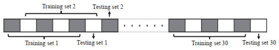
This study randomly selects 30% of the entire data as the parameter setting data, which are constructed by extracting the equal proportion of data from each of the 35 days. The proportion of percentage of the increase and decrease instances in each day is also maintained. Such parameter setting dataset was further divided into training and hold-out set, each of which consists 15% of the entire data. The above procedures were repeated 20 times to construct 20 parameter setting dataset and the optimal combination of parameters was obtained by averaging over the experimental performance on all the sets.
Our study uses an overlapping rolling-forward training and testing procedure. Namely, we subsequently use one week of data for training a model and the following day of data for testing. Similar processes can be found in [
4,
18,
19]. Thus we have thirty training-testing datasets, each of which consists 1200 instances as training data and 240 instances as testing data. The dataset separation is shown in
Figure 1.
Figure 1 The rolling-forward data separation scheme |
Full size|PPT slide
3.2 Procedures
Previous studies such as [
4,
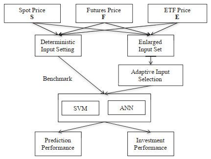
6] use deterministic input sets for high-frequency stock trend prediction, where parametrized technical indicators remain the same as dataset varies. We propose to adaptively select the optimal period parameters through feature selection techniques for the indicators as the market pattern changes, and a prediction model can have different input variables when applied to various dataset. To evaluate the performance of this adaptive input selection (AIS) approach, we incorporate it into machine learners to predict the 5-minute ahead CSI 300 index and compare it with the deterministic input setting (DIS) approach.
For the DIS approach, we adopt deterministic period parameter setting as in [
4], which constitutes a total of 23 variables computed from 8 technical indicators for a time series. These indicators and their period parameters remain the same as dataset varies, which is exhibited in
Table 2. Then a deterministic input set can be the set of variables extracted from S only, S and F, S and E, or all the three series of CSI 300 index.
Table 2 Technical indicators and their formulas |
| Name of indicator | Formula | Period |
| Relative difference prices | RDP$(k) = \frac{p_t-p_{t-k}}{p_{t-k}}\times100$ | 1–3, 5, 10, 20 |
| Moving average (MA) | MA$(k)=\frac{\sum_{i=0}^{k-1}p_{t-i}}{k}$ | 5, 10, 20 |
| Exponential MA | EMA$(k)= \frac{2}{k+1}\sum_{i=0}^k(\frac{k-1}{k+1})^ip_{t-i}$ | 5, 10, 20 |
| Disparity with MA | DISP$(k) = \frac{p_t-{\rm MA}(k)}{{\rm MA}(k)}\times100$ | 5, 10, 20 |
| Disparity with EMA | EDISP$(k) = \frac{p_t-{\rm EMA}(k)}{{\rm EMA}(k)}\times100$ | 5, 10, 20 |
| Oscillator with MA | OSCP$(k, l) = \frac{{\rm MA}(i)-{\rm MA}(j)}{{\rm MA}(i)}$ | (5, 10) |
| Oscillator with EMA | EOSCP$(k, l) = \frac{{\rm EMA}(i) - {\rm EMA}(j)}{{\rm EMA}(i)}$ | (5, 10) |
| Relative strength index | RSI$(k) =\sum_{i=0}^{k-1} \frac{u_{t-i}}{k}/(\sum_{i=0}^{k-1}\frac{d_{t-i}}{k})$ | 5, 10, 20 |
| In RSI, $ u_t $ and $ d_t $ are the upward and downward price change respectively at time $ t $. |
For the AIS approach where input set are adaptively selected to suit time-varying datasets, period parameters for the eight indicators are not restricted as in Table 2. Instead, parameter $ k $ in $ RDP(k) $, $ MA(k) $, $ EMA(k) $, $ DISP(k) $, $ EDISP(k) $ and $ RSI(k) $ are allowed to take on any values interior to 20 and $ (k, l) $ in $ OSCP(k, l) $ and $ EOSCP(k, l) $ to take on (5, 10), (5, 15) and (5, 20). We thus have an enlarged variable set with 116 elements for a time series. Then an adaptive input set can be a subset of the enlarged variable set extracted from S only, S and F, S and E, or all the three series of CSI 300 index.
Each variable in both input sets is then normalized by subtracting the mean over all training values, dividing by the corresponding standard deviation and scaling into the range of $ [-1, 1] $. Due to the page limitation, we show in Tables 3, 4, 5 the summary statistics for some of the input variables extracted from the spot, future and ETF price (S, F and E series) of CSI 300 index as examples. The output variable is a binary variable that if RDP$ (-\Delta 5) $ is positive or zero, then 1, otherwise 0.
Table 3 Summary statistics for some of the inputs in the spot dataset |
| Indicator | Max | Min | Mean | Std |
| RDP(5) | 0.0091 | -0.0064 | 0.0000 | 0.0009 |
| MA(5) | 3552 | 3274 | 3377 | 64.31 |
| EMA(5) | 3552 | 3275 | 3377 | 64.31 |
| DISP(5) | 0.0072 | -0.0033 | 0.0000 | 0.0004 |
| EDISP(5) | 0.0060 | -0.0027 | 0.0000 | 0.0003 |
| OSCP(5, 10) | 0.0040 | -0.0025 | 0.0000 | 0.0004 |
| EOSCP(5, 10) | 0.0020 | -0.0019 | 0.0000 | 0.0003 |
| RSI(5) | 1.0000 | 0.0000 | 0.5077 | 0.3595 |
Table 4 Summary statistics for some of the inputs in the future dataset |
| Indicator | Max | Min | Mean | Std |
| RDP(5) | 0.0110 | -0.0092 | 0.0000 | 0.0010 |
| MA(5) | 3541 | 3269 | 3365 | 62.79 |
| EMA(5) | 3541 | 3270 | 3365 | 62.78 |
| DISP(5) | 0.0080 | -0.0073 | 0.0000 | 0.0005 |
| EDISP(5) | 0.0067 | -0.0061 | 0.0000 | 0.0004 |
| OSCP(5, 10) | 0.0048 | -0.0044 | 0.0000 | 0.0004 |
| EOSCP(5, 10) | 0.0026 | -0.0023 | 0.0000 | 0.0003 |
| RSI(5) | 1.0000 | 0.0000 | 0.5027 | 0.2630 |
Table 5 Summary statistics for some of the inputs in the ETF dataset |
| Indicator | Max | Min | Mean | Std |
| RDP(5) | 0.0094 | -0.0079 | 0.0000 | 0.0009 |
| MA(5) | 3.6138 | 3.3368 | 3.4358 | 0.0644 |
| EMA(5) | 3.6124 | 3.3386 | 3.4358 | 0.0644 |
| DISP(5) | 0.0062 | -0.0036 | 0.0000 | 0.0004 |
| EDISP(5) | 0.0052 | -0.0031 | 0.0000 | 0.0004 |
| OSCP(5, 10) | 0.0039 | -0.0030 | 0.0000 | 0.0004 |
| EOSCP(5, 10) | 0.0021 | -0.0019 | 0.0000 | 0.0003 |
| RSI(5) | 1.0000 | 0.0000 | 0.5016 | 0.3122 |
We use SVM and ANN as the prediction models to compare between DIS and AIS approach. For SVM, Gaussian radial basis function $ k(x_i, x_j) = \exp(-g\|x_i-x_j\|^2) $ is used, where we select the best combination of regularization parameter $ c $ and scaling parameter $ g $ from $ c = 1, 5, 10, 20, 50 $ and $ g = 0.5, 1, 5, 10, 20 $ based on the prediction performance measure on parameter setting dataset. For ANN, we allow the momentum $ mc $ and the number of neurons $ n $ to take values on $ mc = 0.1, 0.2, \cdots, 0.9 $ and $ n = 1, 2, \cdots, 10 $. We then compare AIS with DIS approach through two phases of experiments. In the first phase, we apply SVM or ANN to the 30 datasets with a DIS approach as defined above. In the second phase, we use the AIS approach to select the most suitable period parameters and indicators for each of the 30 time-varying datasets from an enlarged input set. Four types of feature selection techniques, including $ t $-statistics, information gain, ROC and PCA, are tested in the AIS approach. After obtaining the rankings of the features or transformed features, we select the top ranked number of features from 10 to 110 and input them into SVM or ANN to make prediction.
Finally, from the perspective of investment strategy, we evaluate the profitability of a stock trend prediction method based on a virtual trading strategy. It decides to buy at $ T $ and sell at $ T+5 $ if the prediction of the instance at $ T $ is "increase", while decides to sell at $ T $ and buy back at $ T+5 $ if the prediction of the instance at $ T $ is "decrease". Then the accumulated return over all instance is computed as the daily return. The average return and the total return of each of these daily returns are reported in our study.
The whole procedure is shown in Figure 2.
Figure 2 This figure displays the whole procedure of our experiment |
Full size|PPT slide
4 Experimental Results
The first phase of experimentation considers DIS approach. The best combination of parameters for SVM is identified by averaging over experimental results on the 20 randomly selected parameter setting datasets. Since the prediction accuracy and F-measure don't always reach the optimal value simultaneously, we choose the parameter combination with the highest accuracy measure restricted to the condition that the corresponding F-measure is above the top 25%. For SVM, the accuracy and F-measure are not very sensitive to the change of input variables. The best parameters of SVM are $ c=20 $ and $ g=5 $. For ANN, the best combinations of parameters vary as the input information changes. The selected parameters for SVM and ANN on four types of input information are reported in Table 6.
Table 6 Best parameter combinations of SVM and ANN on parameter setting dataset |
| | | S | SF | SE | SFE |
| SVM | Param. | c: 20, g: 5 | c: 20, g: 5 | c: 20, g: 5 | c: 20, g: 5 |
| Accu. | 0.6027 | 0.6284 | 0.6008 | 0.6324 |
| F-meas. | 0.6011 | 0.6311 | 0.6006 | 0.6362 |
| ANN | Param. | n: 8, mc: 0.8 | n: 4, mc: 0.7 | n: 4, mc: 0.6 | n: 9, mc: 0.4 |
| Accu. | 0.5972 | 0.6222 | 0.5961 | 0.6216 |
| F-meas. | 0.6143 | 0.6333 | 0.6088 | 0.6357 |
Then we apply SVM or ANN, parametrized by the selected parameter combinations, to the 30 datasets using the DIS approach. The best performance of SVM and ANN is reported in Table 7. The highest performance achieved by different types of information inputs is boldfaced for each method.
Table 7 Performance of SVM and ANN with DIS approach |
| | | S | SF | SE | SFE |
| SVM | Accu. | 0.6128 | 0.6196 | 0.6118 | 0.6160 |
| F-meas. | 0.6165 | 0.6236 | 0.6187 | 0.6204 |
| ANN | Accu. | 0.5932 | 0.6096 | 0.5899 | 0.6125 |
| F-meas. | 0.6202 | 0.6107 | 0.6064 | 0.6269 |
In the second phase of our experiment, we use the AIS method as explained in Section 3.2 to select the most suitable inputs for each dataset. For every kind of information extracted from S, SF, SE or SFE series, four feature selection techniques including $ t $-statistics, information gain, ROC and PCA, are applied to adaptively rank the enlarged input sets (defined in Section 3.2). We then select the number of top ranked input variables, based on the ranking results of each feature selection techniques, from 10 to 110 (with an interval of 10) as inputs to SVM or ANN. We still use the optimal parameter combinations of SVM and ANN reported in Table 6 for each kind of input information. The best performance of SVM and ANN with AIS approach is reported respectively in Tables 8 and 9. The highest performance achieved by each method is boldfaced.
Table 8 Performance of SVM with AIS approach |
| | S | SF | SE | SFE |
| T-stat | Accu. | 0.6193 | 0.6356 | 0.6200 | 0.6381 |
| F-meas. | 0.6280 | 0.6449 | 0.6257 | 0.6467 |
| IG | Accu. | 0.6169 | 0.6317 | 0.6190 | 0.6307 |
| F-meas. | 0.6303 | 0.6433 | 0.6274 | 0.6410 |
| ROC | Accu. | 0.6149 | 0.6332 | 0.6161 | 0.6315 |
| F-mea. | 0.6245 | 0.6373 | 0.6176 | 0.6399 |
| PCA | Accu. | 0.6153 | 0.6188 | 0.6153 | 0.6188 |
| F-meas. | 0.6248 | 0.6287 | 0.6248 | 0.6287 |
Table 9 Performance of ANN with AIS approach |
| | S | SF | SE | SFE |
| T-stat | Accu. | 0.6189 | 0.6263 | 0.6258 | 0.6310 |
| F-meas. | 0.6257 | 0.6455 | 0.6377 | 0.6438 |
| IG | Accu. | 0.6119 | 0.6299 | 0.6071 | 0.6288 |
| F-meas. | 0.6233 | 0.6451 | 0.6323 | 0.6490 |
| ROC | Accu. | 0.6115 | 0.6272 | 0.6054 | 0.6271 |
| F-meas. | 0.6223 | 0.6400 | 0.6121 | 0.6403 |
| PCA | Accu. | 0.6158 | 0.6185 | 0.6015 | 0.6149 |
| F-meas. | 0.6282 | 0.6196 | 0.6216 | 0.6321 |
Comparing to Table 7, the results show that the best performance of AIS approach using respectively $ t $-statistics, information gain and ROC method have comparably values, which is better than that of DIS approach. For SVM, the highest prediction accuracy of 63.81% and F-measure of 64.67% with AIS approach are respectively 1.85% and 2.31% higher than that with DIS approach. Since the standard deviation of the prediction error based on the 30 datasets with 240 samples per set should around $ \sqrt{63.81\%\times(1-63.81\%)/(30\times 240)} = 0.56\% $ and $ \sqrt{64.67\%\times(1-64.67\%)/(30\times 240)} = 0.56\% $, the improvement in prediction accuracy and F-measure of AIS over DIS is very significant. For ANN, the highest prediction accuracy and F-measure with AIS are 63.10% and 64.38% respectively, which are also significantly higher than 60.96% and 61.07% for DIS. It is also observed that PCA technique performs poorly to select discriminating input sets, which shows no significant improvement with any types of information inputs comparing to DIS. This might indicate that the new combination of indicators constructed by PCA is not as informative as the original ones for high-frequency stock prediction.
Furthermore, we notice that the best performance is always obtained on any input sets that include the futures price of CSI 300 index whenever the input set is deterministic or adaptive. This implies that futures information is very helpful in predicting the trends of the spot price of CSI 300 index. By using the $ t $-statistics method to adaptively select the inputs to SVM and ANN, the best performance is obtained with all the information from the spot, futures and ETF series of CSI 300 index. This implies that the ETF series provides additional information for the prediction of the CSI 300 index. But such information helps very little to predict CSI 300 index since the performance of both SVM and ANN with SFE information is only slightly better than that with SF information.
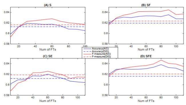
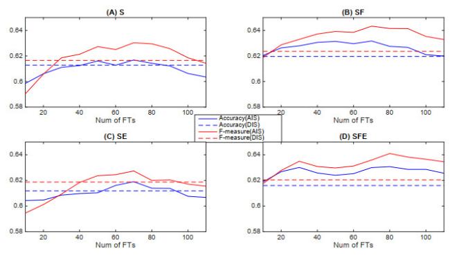
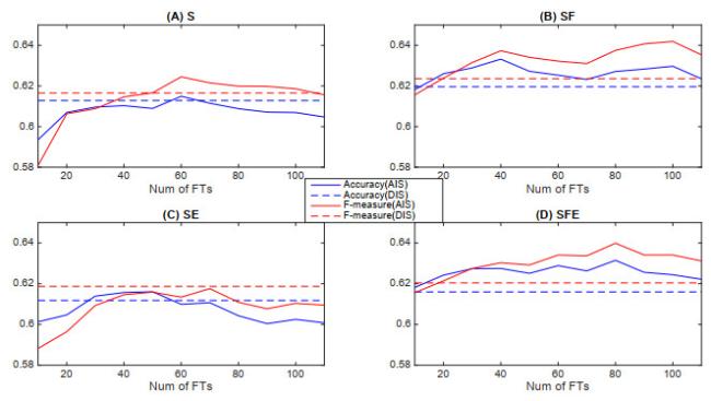
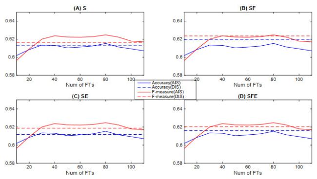
Because of the page limitation, we show respectively in Figures 3, 4, 5, 6 only the prediction performance of SVM with AIS approach over the 30 datasets. The solid lines in each figure represent the prediction performance with each of the AIS methods for a certain type of information input (information from S, SF, SE or SFE series). The dashed lines exhibit the prediction performance with the DIS approach as benchmarks. Firstly, it is observed that the AIS by $ t $-statistics and information gain can achieve better performance than DIS on some sizes of selected input sets with all four kinds of information input. The performance improvement with any information input that includes futures price is significant and can be obtained on almost all input sizes between 20 to 110. Secondly, we observe that there is no performance improvement for ROC feature selection without futures information while significant improvement can be obtained by ROC feature selection with SF or SFE information. Finally, it is observed that there is slightly or no significant improvement in performance for PCA feature selection technique with any types of information inputs.
Figure 3 Performance of SVM with AIS approach using $t$-statistics |
Full size|PPT slide
Figure 4 Performance of SVM with AIS approach using information gain |
Full size|PPT slide
Figure 5 Performance of SVM with AIS approach using ROC |
Full size|PPT slide
Figure 6 Performance of SVM with AIS approach using PCA |
Full size|PPT slide
In the end, we compare the investment performance of the AIS approach using the three well-performed feature selection methods ($ t $-statistics, information gain and ROC) with that of the DIS approach. For the DIS approach, we use the whole deterministic input set extracted from the spot and futures prices of CSI 300 index since this combination of information inputs gives the best prediction results. For each of the AIS approaches, we use the information set and the number of input variables that give the best prediction accuracy. The settings of the methods, the daily and the total returns within the 30 testing days are presented in Table 10. It is observed that the AIS approach using the three methods can give the better returns than DIS approach.
Table 10 Virtual trading returns with DIS and AIS approaches |
| | DIS | AIS-T-stat | AIS-IG | AIS-ROC |
| SVM | FT Set | SF | SFE | SF | SF |
| Num of FTs | 69 | 80 | 70 | 40 |
| Daily Return | 0.0198 | 0.0199 | 0.0205 | 0.0229 |
| Total Return | 0.5930 | 0.5970 | 0.6161 | 0.6883 |
| ANN | FT Set | SF | SFE | SF | SF |
| Num of FTs | 69 | 80 | 40 | 70 |
| Daily Return | 0.0168 | 0.0223 | 0.0214 | 0.0202 |
| Total Return | 0.5036 | 0.6703 | 0.6406 | 0.6047 |
5 Conclusion
In this paper, we compare the adaptive input selection (AIS) approach with the deterministic input setting (DIS) approach for the 5-minute ahead prediction of CSI 300 index movements in Chinese stock market. We use support vector machines (SVM) and artificial neural networks (ANN) to train prediction models and use the eight technical indicators in [
4] to construct the input set. In the DIS approach, we apply the original period parameter setting for the indicators as in [
4]. To implement the AIS approach, the period parameters for the technical indicators are allowed to take on a wide range of numbers, while the optimal sets of indicators and their suitable period parameters are adaptively selected for the time-varying dataset. Four feature selection methods, including
$ t $-statistics, information gain, ROC and PCA, are used in the AIS approach. The results show that the AIS approach with
$ t $-statistics, information gain and ROC can achieve significantly better prediction performance than the DIS approach. But there are no significant differences in the prediction performance between the AIS approach with PCA and DIS approaches. When a virtual trading strategy is applied to evaluate the profitability of each method, the AIS approach with
$ t $-statistics, information gain and ROC also show better results than the DIS approach. These conclusions should be helpful for traders or researchers who are interested in high-frequency stock prediction.
{{custom_sec.title}}
{{custom_sec.title}}
{{custom_sec.content}}
 PDF(191 KB)

 Table 1 The percentage of increase cases in each day in the entire dataset
 Figure 1 The rolling-forward data separation scheme


