Moving Average Model with an Alternative GARCH-Type Error

Huafeng ZHU; Xingfa ZHANG; Xin LIANG; Yuan LI

doi:10.21078/JSSI-2018-165-13

PDF(171 KB)

Journal of Systems Science and Information ›› 2018, Vol. 6 ›› Issue (2) : 165-177. DOI: 10.21078/JSSI-2018-165-13

Moving Average Model with an Alternative GARCH-Type Error

Author information +

History +

Abstract

Motivated by the double autoregressive model with order $p$ (DAR( $p$ ) model), in this paper, we study the moving average model with an alternative GARCH error. The model is an extension from DAR( $p$ ) model by letting the order $p$ goes to infinity. The quasi maximum likelihood estimator of the parameters in the model is shown to be asymptotically normal, without any strong moment conditions. Simulation results confirm that our estimators perform well. We also apply our model to study a real data set and it has better fitting performance compared to DAR model for the considered data.

Key words

moving average model / double autoregressive model / quasi maximum likelihood estimator

Cite this article

EndNote

Ris (Procite)

Bibtex

Download Citations

Huafeng ZHU , Xingfa ZHANG , Xin LIANG , Yuan LI. Moving Average Model with an Alternative GARCH-Type Error. Journal of Systems Science and Information, 2018, 6(2): 165-177 https://doi.org/10.21078/JSSI-2018-165-13

1 Introduction

Consider the DAR

(p)

model with the form

y_{t} = \sum_{i = 1}^{p} ϕ_{i} y_{t - i} + η_{t} \sqrt{ω + \sum_{i = 1}^{p} α_{i} y_{t - i}^{2}},

(1)

where

ω, α_{i} > 0

t \in N \equiv {1, 2, \dots}

{η_{t}}

is an independent identically distributed sequence with mean

0

and variance

1

, and

y_{s}

is independent of

{η_{t} : t \geq 1}

for

s \leq 0

. Let

F_{t}

be the

σ -

field generated by

{η_{t}, η_{t - 1}, \dots, η_{1}, y_{0}, y_{- 1}, \dots, y_{1 - p}}, t \in N

. Given

F_{t - 1}

, the conditional variance of

y_{t}

var (y_{t} | F_{t - 1}) = ω + \sum_{i = 1}^{p} α_{i} y_{t - i}^{2}

. Compared to the classic autoregressive (AR) model, it is found, by Ling^{[1, 2]}, that DAR

(p)

model has the following novelty: even some roots of

1 - \sum_{i = 1}^{p} ϕ_{i} z^{i} = 0

are on or outside the unit circle, and for the case

E y_{t}^{2} = \infty

, the quasi maximum likelihood estimator (QMLE) for DAR

(p)

model is still asymptotically normal, which does not hold for classic AR(

p

) model with i.i.d. errors. Due to the novelty and simplicity of DAR models, many extensions have been done based on Ling^[2]. For example, Ling and Li^[3] and Chen, et al.^[4] considered the asymptotic inference for nonstationary DAR model; Kwok and Li^[5] investigated the diagnostic checking of the DAR model; Liu^[6] studied the structure of a DAR process driven by a hidden Markov chain; Cai, et al.^[7] proposed the quantile DAR models for financial returns; Zhu and Ling^[8] gave asymptotic theory of quasi maximum exponential likelihood estimation for DAR model; Guo, et al.^[9] proposed a factor DAR models with application to simultaneous causality testing. Other extensions can be referred to threshold DAR models by Zhang, et al.^[10], Li, et al.^[11] and Li, et al.^[12]; mixture DAR model by Li, et al.^[13], and explosive DAR model by Liu, et al.^[14].

While, to the best of our knowledge, few work has been done to discuss the question that: how to set

p

goes to

\infty

for Model (1)? Undoubtedly, the question is interesting because more information will be used for statistical inference. Directly setting

p = \infty

in Model (1) is not feasible due to complexity. Fortunately, like ARCH(

p

) model (Engle^[15]) being extended to GARCH model (Bollerslev^[16]), the above question can be partially solved in an indirect way. Motivated by the moving average (MA) model and new GARCH specification adopted by Christensen, et al.^[17], we consider the following moving average model with an alternative GARCH error

\begin{array}{rcl} y_{t} = ϕ ε_{t - 1} + ε_{t}, \end{array}

(2)

\begin{array}{rcl} ε_{t} = η_{t} \sqrt{h_{t}}, \end{array}

(3)

\begin{array}{rcl} h_{t} = ω + α y_{t - 1}^{2} + β h_{t - 1}, \end{array}

(4)

where,

| ϕ | < 1, ω, α > 0, 0 < β < 1

{η_{t}}

is an independent identically distributed sequence with mean

0

and variance

1

, and

y_{s}

is independent of

{η_{t} : t > s}

. It is seen that Equations (2)–(4) is simply the MA(1) model with an error term whose conditional variance is specified as an alternative GARCH form given in (4). Different from the traditional MA-GARCH model, the previous

ε_{t - 1}^{2}

in (4) is instead by

y_{t - 1}^{2}

. Such kind of GARCH specification of (4) has been adopted by several authors such as Christensen, et al.^[17], Zhang, et al.^[18] and Zhang, et al.^[19]. By simple iterations, (2)–(4) can be transformed into the followed form

\begin{array}{rcl} y_{t} = \sum_{i = 1}^{\infty} (- 1)^{i - 1} ϕ^{i} y_{t - i} + η_{t} \sqrt{\frac{ω}{1 - β} + α \sum_{j = 1}^{\infty} β^{j - 1} y_{t - j}^{2}} . \end{array}

(5)

Compared to (1), (5) straightforwardly explains why (2)–(4) can be considered as one kind of DAR(

\infty

) model. Let

F_{t}

be the

σ

-field generated by

{η_{t}, η_{t - 1}, \dots, η_{1}, y_{0}, y_{- 1} \dots}

. Given

F_{t - 1}

, the conditional variance of

y_{t}

in (2) or (5) is

var (y_{t} | F_{t - 1}) = h_{t}

Due to the use of more information, Model (2)–(4) is expected to have a better fitting performance compared to common DAR model with finite order. Another consideration is whether the QMLE of (2)–(4) has similar asymptotic results compared to the case of DAR(

p

) model. In this paper, the above two issues will be investigated. The rest of the paper is organized as follows. In Section 2, we discuss the asymptotic normality of the QMLE for the considered model. Simulations and empirical studies are respectively shown in Section 3 and Section 4. We conclude the article in Section 5 and the proofs are put in the Appendix.

2 Quasi Maximum Likelihood Estimation

Define

θ = (ϕ, ω, α, β)^{τ} \in Θ

. Here

Θ

is a parameter space for Model (2)–(4) with a form

Θ ≜

{

θ

: -1<

\underline{ϕ}

ϕ

\bar{ϕ}

<1,0<

\underline{ω}

ω

\bar{ω}

, 0<

\underline{α}

α

\bar{α}

, 0<

\underline{β}

β

\bar{β}

<1. Suppose that the true parameter, say

θ_{0} = (ϕ_{0}, ω_{0}, α_{0}, β_{0})^{τ}

, is an interior point of the considered parameter space. We need to estimate

θ

based on the observations

{y_{t}}_{t = 1}^{n}

and initial values

y_{0}, h_{0}, ε_{0}

. Following the convention in the literature, we consider the quasi conditional log-likelihood function (apart from a constant term)

L_{n}^{} (θ) = \frac{1}{n} \sum_{t = 1}^{n} l_{t}^{} (θ) = \frac{1}{n} \sum_{t = 1}^{n} {\log h_{t} (θ) + \frac{ε_{t}^{2} (θ)}{h_{t} (θ)}},

(6)

where

ε_{t} (θ) = y_{t} - ϕ ε_{t - 1} (θ)

. Based on

{y_{t}}_{t = 1}^{n}

and initial values, the estimator for

θ

is defined as

{\hat{θ}}_{n} = \arg min_{θ \in Θ} L_{n}^{} (θ) .

(7)

For convenience of notations, we put

\begin{array}{rcl} ς = E η_{t}^{4} - 1, h_{t} = h_{t} (θ_{0}), ε_{t} = ε_{t} (θ_{0}) = y_{t} - ϕ_{0} ε_{t - 1} (θ_{0}), \\ H_{t} = {[\frac{1}{1 - β_{0}}, \sum_{j = 1}^{\infty} β_{0}^{j - 1} y_{t - j}^{2}, \sum_{j = 1}^{\infty} β_{0}^{j - 1} h_{t - j}]}^{τ} . \end{array}

Before stating the asymptotic results for

{\hat{θ}}_{n}

, we firstly make the following assumptions.

(ⅰ) The i.i.d. (0, 1) process

{η_{t}}

satisfies

E (η_{t}^{4}) < \infty

(ⅱ) The series

{y_{t}}

generated from Model (2)–(4) is strictly stationary and geometrically ergodic.

Theorem 1 For Model $(2) - (4)$ and the considered quasi log-likelihood function $L_{n}^{} (θ)$ given by $(6)$ . Suppose Assumptions (ⅰ)–(ⅱ) hold. Then there exists a fixed open neighborhood $U (θ_{0}) \subset Θ$ such that with probability one, as $n \to \infty$ , $L_{n}^{} (θ)$ has an unique minimum point ${\hat{θ}}_{n}$ in $U (θ_{0})$ . Furthermore,

\sqrt{n} ({\hat{θ}}_{n} - θ_{0}) \overset{L}{⟶} N (0, Ω_{I}^{- 1} Ω_{S} Ω_{I}^{- 1}),

where

Ω_{S} = E [\begin{matrix} \frac{4}{h_{t}} {(\sum_{i = 1}^{\infty} (- 1)^{i} i {ϕ_{0}}^{i - 1} y_{t - i})}^{2} & 0 \\ 0 & \frac{ς}{h_{t}^{2}} H_{t} H_{t}^{τ} \end{matrix}],

Ω_{I} = E [\begin{matrix} \frac{2}{h_{t}} {(\sum_{i = 1}^{\infty} (- 1)^{i} i {ϕ_{0}}^{i - 1} y_{t - i})}^{2} & 0 \\ 0 & \frac{1}{h_{t}^{2}} H_{t} H_{t}^{τ} \end{matrix}] .

Remark 1 The proof of Theorem 1 is based on verifying the conditions of Lemma 1 in Jensen and Rahbek^[20]. It can be seen that

E y_{t}^{2} < \infty

is not required to guarantee the validity of the theorem and such a result is consistent with that of DAR(

p

) model in Ling^[2]. In practice, initial values

h_{0}, ε_{0}

are needed to calculate

L_{n} (θ)

and commonly one can set

h_{0} = var (y_{t}), ε_{0} = 0

. The matrices

Ω_{S}, Ω_{I}

can be approximated by the relevant sample means after the parameters

θ = (ϕ, ω, α, β)^{τ}

and

h_{t} (θ)

have been estimated.

3 Simulations

This section examines the performance of the QMLEs through the Monte Carlo experiments. We study the bias and standard deviations of the estimates. The series

y_{t}

is generated through Model (2)–(4) with

η_{t} \sim i . i . d . N (0, 1)

. Noting

θ = (ϕ, ω, α, β)^{τ}

, the following four cases are considered:

\begin{array}{rcl} θ = (0.9, 0.1, 0.3, 0.5)^{τ}, θ = (0.2, 0.1, 0.2, 0.7)^{τ}, \\ θ = (0.1, 0.8, 0.7, 0.1)^{τ}, θ = (- 0.55, 0.8, 0.7, 0.1)^{τ} . \end{array}

The sample sizes are

n = 400

and

n = 800

1000

replications are used. To run the estimation, we set the initial value for the conditional variance

h_{0} = var (y_{t}), ε_{0} = 0

and

θ \in [- 0.99, 0.99] \times [0.001, 1.5] \times [0.001, 0.99] \times [0.001, 0.99]

Table 1 summarizes the empirical biases, empirical standard deviations (SD) and asymptotic standard deviations (AD) of the QMLEs of

θ = (ϕ, ω, α, β)^{τ}

. The ADs are calculated according to Theorem 1 and its remark. Table 1 shows that all the biases of the QMLEs are very small. It can be seen that the SDs and ADs are very close. As the sample size

n

is increased from 400 to 800, all SDs and ADs become smaller. The simulation results indicate that the QMLE performs well.

Table 1 Bias and standard deviations of QMLEs

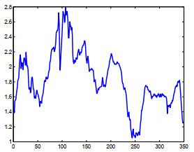
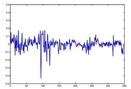
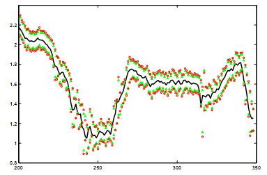
$θ = (ϕ, ω, α, β)^{τ}$		$\hat{ϕ}$	$\hat{ω}$	$\hat{α}$	$\hat{β}$
$(0.9, 0.1, 0.3, 0.5)^{τ}$	Bias	$-$ 0.0047	0.0148	0.0038	$-$ 0.0157
$(n = 400)$	SD	0.0229	0.0717	0.0614	0.0712
	AD	0.0179	0.0259	0.0481	0.0515
$(0.9, 0.1, 0.3, 0.5)^{τ}$	Bias	$-$ 0.0027	0.0077	0.0034	$-$ 0.0089
$(n = 800)$	SD	0.0155	0.0535	0.0462	0.0498
	AD	0.0125	0.0213	0.0388	0.0412
$(0.2, 0.1, 0.2, 0.7)^{τ}$	Bias	0.0013	0.0243	$-$ 0.0016	$-$ 0.0286
$(n = 400)$	SD	0.0537	0.0739	0.0595	0.1082
	AD	0.0548	0.0384	0.0556	0.0680
$(0.2, 0.1, 0.2, 0.7)^{τ}$	Bias	0.0011	0.0101	0.0006	$-$ 0.0131
$(n = 800)$	SD	0.0384	0.0354	0.0390	0.0591
	AD	0.0386	0.0321	0.0395	0.0629
$(0.1, 0.8, 0.7, 0.1)^{τ}$	Bias	$-$ 0.0009	0.0223	$-$ 0.0119	$-$ 0.0076
$(n = 400)$	SD	0.0678	0.1475	0.1108	0.0633
	AD	0.0617	0.1239	0.1071	0.0495
$(0.1, 0.8, 0.7, 0.1)^{τ}$	Bias	0.0019	0.0105	$-$ 0.0078	$-$ 0.0020
$(n = 800)$	SD	0.0455	0.1078	0.0850	0.0491
	AD	0.0462	0.0840	0.0820	0.0435
$(- 0.55, 0.8, 0.7, 0.1)^{τ}$	Bias	0.0018	0.0217	$-$ 0.0052	$-$ 0.0049
$(n = 400)$	SD	0.0385	0.1500	0.1055	0.0539
	AD	0.0359	0.1345	0.0908	0.0400
$(- 0.55, 0.8, 0.7, 0.1)^{τ}$	Bias	$-$ 0.0005	0.0048	$-$ 0.0032	$-$ 0.0010
$(n = 800)$	SD	0.0267	0.1020	0.0724	0.0363
	AD	0.0245	0.0897	0.0693	0.0204

†Number of replications=1000.

4 Empirical Studies

In this section, Model (2)–(4) is applied to study a real data set. We analyze the US monthly interest rate series over the period July 1972–August 2001. The series is the 90-day treasury bill rate and has 350 observations in total. Such a data set has also been analyzed by Ling^[1]. Take

x_{t}

to be the logarithms of the 90-day treasury bill rate and

y_{t} = x_{t} - x_{t - 1}

. We plot

x_{t}

and

y_{t}

in Figs 1 and 2 respectively.

Figure 1 Time plot of $x_{t}$ (logarithms of the US 90-day treasury bill rate)

Full size|PPT slide

Figure 2 Time plot of $y_{t}$ ( $y_{t} = x_{t} - x_{t - 1}$ )

Full size|PPT slide

DAR(1) model has been adopted to fit

y_{t}

by Ling^[1] and the result is

\begin{array}{rcl} y_{t} = {0.3810}_{(0.0777)} y_{t - 1} + ε_{t}, \\ ε_{t} = η_{t} \sqrt{{{0.0023}_{(0.0002)} + {0.6209}_{(0.0908)} y_{t - 1}^{2}}}, \end{array}

(8)

where the values in parentheses are the corresponding standard deviations.

Similarly, we also use Model (2)–(4) to fit series

{y_{t}}

and the result is

\begin{array}{rcl} y_{t} = {0.4065}_{(0.0575)} ε_{t - 1} + ε_{t}, ε_{t} = η_{t} \sqrt{h_{t}}, \\ h_{t} = {0.0010}_{(0.0003)} + {0.4339}_{(0.1246)} y_{t - 1}^{2} + {0.2823}_{(0.1291)} h_{t - 1}, \end{array}

(9)

where the standard deviations in parentheses are calculated based on Theorem 1.

To compare, for Models (8)–(9), root of mean squared error (RMSE) for one-step-ahead forecast and value of the log-likelihood are respectively listed in Table 2. Further, Figure 3 shows time plots of data

x_{t}

with

95 %

confidence intervals for the one-step-ahead forecast based on (8)–(9), starting from February 1989. It is shown that the confidence intervals based on Model (9) are narrower than those based on (8) at nearly all the data points. From Table 2 and Figure 3, Model (9) is superior to the DAR(1) model.

Table 2 Fitting performance for Models (8)–(9)

Model	RMSE for one-step-ahead forecast	Log-likelihood value
(8)	0.0590	764.4363
(9)	0.0583	780.5071

Figure 3 Plot of the data $x_{t}$ (real line), $95 %$ forecasting confidence intervals based on Model (8) (circle) and (9) (triangle) respectively

Full size|PPT slide

5 Conclusions

With the motivation to study the DAR(

p

) model with

p

going to

\infty

, in this article, we propose a special moving average model with an alternative GARCH-type error. Asymptotic normality for QMLE of the model is established under weak conditions. Through the simulations, it is found that the estimation performs well. Empirical study shows the considered model can have better fitting performance compared to the previous DAR model. This implies our model framework can be used for potential applications where a DAR model structure is applicable.

Appendix

Lemma 1 (Lemma 1 of Jensen and Rahbek^[20]) Denote $L_{n} (θ)$ as a function of the observations $y_{1}, y_{2}, \dots, y_{n}$ and the parameter $θ \in Θ \subseteq R^{k}$ . Suppose $θ_{0}$ is an interior point of $Θ$ . Assume $L_{n} (.) : R^{k} \to R$ is three times continuously differentiable in $θ$ and

(ⅰ) As $n \to \infty$ , $\sqrt{n} \frac{\partial L_{n} (θ_{0})}{\partial θ} \overset{L}{\to} N (0, Ω_{S}), Ω_{S} > 0$ ;

(ⅱ) As $n \to \infty$ , $\frac{\partial^{2} L_{n} (θ_{0})}{\partial θ \partial θ^{τ}} \overset{P}{\to} Ω_{I} > 0$ ;

(ⅲ)

max_{i, j, k = 1, 2, \dots, p + 2} sup_{θ \in N (θ_{0})} | \frac{\partial^{3} L_{n} (θ_{0})}{\partial θ_{i} \partial θ_{j} \partial θ_{k}} | \leq c_{n}, 0 \leq c_{n} \overset{P}{\to} c < \infty .

Here, $N (θ_{0})$ is a neighborhood of $θ_{0}$ . Then there exists a fixed open neighborhood $U (θ_{0}) \subseteq N (θ_{0})$ such that:

(ⅰ) As $n \to \infty$ , with probability one that there exists a minimum point ${\hat{θ}}_{n}$ of $L_{n} (θ)$ in $U (θ_{0})$ and $L_{n} (θ)$ is convex in $U (θ_{0})$ . Moreover, ${\hat{θ}}_{n}$ is unique and solves $\frac{\partial L_{n} ({\hat{θ}}_{n})}{\partial θ} = 0$ ;

(ⅱ) As $n \to \infty$ , ${\hat{θ}}_{n} - θ_{0} \overset{P}{\to} 0$ , $\sqrt{n} ({\hat{θ}}_{n} - θ_{0}) \overset{L}{\to} N (0, Ω_{I}^{- 1} Ω_{S} Ω_{I}^{- 1}) .$

Before giving proof for Theorem 1, we need to state some expressions and one lemma. Let symbol variables

s_{1}, s_{2}, s_{3}

take values from symbol set

{i, j, k} .

In terms of (6), it is not difficult to get the derivatives of the quasi log-likelihood function with respect to

θ

\frac{\partial l_{t}^{} (θ)}{\partial θ} = (1 - \frac{ε_{t}^{2} (θ)}{h_{t} (θ)}) \frac{1}{h_{t} (θ)} \frac{\partial h_{t} (θ)}{\partial θ} + \frac{2 ε_{t} (θ)}{h_{t} (θ)} \frac{\partial ε_{t} (θ)}{\partial θ},

(A.1)

\begin{array}{lll} \frac{\partial^{2} l_{t}^{} (θ)}{\partial θ \partial θ^{τ}} & = & - \frac{1}{h_{t}^{2} (θ)} (1 - \frac{2 ε_{t}^{2} (θ)}{h_{t} (θ)}) \frac{\partial h_{t} (θ)}{\partial θ} \frac{\partial h_{t} (θ)}{\partial θ^{τ}} - \frac{2 ε_{t} (θ)}{h_{t}^{2} (θ)} \frac{\partial h_{t} (θ)}{\partial θ} \frac{\partial ε_{t} (θ)}{\partial θ^{τ}} \\ + \frac{2}{h_{t} (θ)} \frac{\partial ε_{t} (θ)}{\partial θ} \frac{\partial ε_{t} (θ)}{\partial θ^{τ}} + \frac{2 ε_{t} (θ)}{h_{t} (θ)} \frac{\partial^{2} ε_{t} (θ)}{\partial θ \partial θ^{τ}} \\ - \frac{2 ε_{t} (θ)}{h_{t}^{2} (θ)} \frac{\partial ε_{t} (θ)}{\partial θ} \frac{\partial h_{t} (θ)}{\partial θ^{τ}} + \frac{1}{h_{t} (θ)} (1 - \frac{ε_{t}^{2} (θ)}{h_{t} (θ)}) \frac{\partial^{2} h_{t} (θ)}{\partial θ \partial θ^{τ}}, \end{array}

(A.2)

\frac{\partial^{3} l_{t}^{} (θ)}{\partial θ_{i} \partial θ_{j} \partial θ_{k}} = d_{1 t} (θ) + d_{2 t} (θ) + d_{3 t} (θ),

(A.3)

where,

\begin{array}{lll} d_{1 t} (θ) & = & - \frac{2 (h_{t} (θ) - 3 ε_{t}^{2} (θ))}{h_{t}^{4} (θ)} \frac{\partial h_{t} (θ)}{\partial θ_{i}} \frac{\partial h_{t} (θ)}{\partial θ_{j}} \frac{\partial h_{t} (θ)}{\partial θ_{k}} \\ + \frac{2 ε_{t} (θ)}{h_{t}^{3} (θ)} \sum_{s_{1} \neq s_{2} \neq s_{3}} \frac{\partial h_{t} (θ)}{\partial θ_{s_{1}}} \frac{\partial h_{t} (θ)}{\partial θ_{s_{2}}} \frac{\partial ε_{t} (θ)}{\partial θ_{s_{3}}} \\ - \frac{1}{h_{t}^{2} (θ)} \sum_{s_{1} \neq s_{2} \neq s_{3}} \frac{\partial h_{t} (θ)}{\partial θ_{s_{1}}} \frac{\partial ε_{t} (θ)}{\partial θ_{s_{2}}} \frac{\partial ε_{t} (θ)}{\partial θ_{s_{3}}}, \end{array}

(A.4)

\begin{array}{lll} d_{2 t} (θ) & = & \frac{1}{h_{t}^{2} (θ)} (\frac{ε_{t}^{2} (θ)}{h_{t} (θ)} - 1) \sum_{s_{1} \neq s_{2} \neq s_{3}} \frac{\partial h_{t} (θ)}{\partial θ_{i}} \frac{\partial^{2} h_{t} (θ)}{\partial θ_{s_{2}} \partial θ_{s_{3}}} \\ - \frac{ε_{t} (θ)}{h_{t}^{2} (θ)} \sum_{s_{1} \neq s_{2} \neq s_{3}} \frac{\partial h_{t} (θ)}{\partial θ_{s_{1}}} \frac{\partial^{2} ε_{t} (θ)}{\partial θ_{s_{2}} \partial θ_{s_{3}}} \\ - \frac{ε_{t} (θ)}{h_{t}^{2} (θ)} \sum_{s_{1} \neq s_{2} \neq s_{3}} \frac{\partial ε_{t} (θ)}{\partial θ_{s_{1}}} \frac{\partial^{2} h_{t} (θ)}{\partial θ_{s_{2}} \partial θ_{s_{3}}} \\ + \frac{1}{h_{t} (θ)} \sum_{s_{1} \neq s_{2} \neq s_{3}} \frac{\partial ε_{t} (θ)}{\partial θ_{s_{1}}} \frac{\partial^{2} ε_{t} (θ)}{\partial θ_{s_{2}} \partial θ_{s_{3}}}, \end{array}

(A.5)

d_{3 t} (θ) = \frac{1}{h_{t} (θ)} (1 - \frac{ε_{t}^{2} (θ)}{h_{t} (θ)}) \frac{\partial^{3} h_{t} (θ)}{\partial θ_{i} \partial θ_{j} \partial θ_{k}} + \frac{2 ε_{t} (θ)}{h_{t} (θ)} \frac{\partial^{3} ε_{t} (θ)}{\partial θ_{i} \partial θ_{j} \partial θ_{k}} .

(A.6)

Simple calculations gives

\begin{array}{rcl} ε_{t} (θ) = y_{t} - ϕ ε_{t - 1} (θ) = \sum_{i = 0}^{\infty} (- 1)^{i} ϕ^{i} y_{t - i}, \end{array}

(A.7)

\begin{array}{rcl} \frac{\partial ε_{t} (θ)}{\partial ω} = \frac{\partial ε_{t} (θ)}{\partial α} = \frac{\partial ε_{t} (θ)}{\partial β} = 0, \frac{\partial ε_{t} (θ)}{\partial ϕ} = \sum_{i = 1}^{\infty} (- 1)^{i} i ϕ^{i - 1} y_{t - i}, \end{array}

(A.8)

\begin{array}{rcl} \frac{\partial^{2} ε_{t} (θ)}{\partial ϕ^{2}} = \sum_{i = 2}^{\infty} (- 1)^{i} i (i - 1) ϕ^{i - 2} y_{t - i}, \end{array}

(A.9)

\begin{array}{rcl} \frac{\partial^{3} ε_{t} (θ)}{\partial ϕ^{3}} = \sum_{i = 3}^{\infty} (- 1)^{i} i (i - 1) (i - 2) ϕ^{i - 3} y_{t - i} . \end{array}

(A.10)

Similarly, one can get

\begin{array}{rcl} h_{t} (θ) = \frac{ω}{1 - β} + α \sum_{j = 0}^{\infty} β^{j} y_{t - j - 1}^{2}, \end{array}

(A.11)

\begin{array}{rcl} \frac{\partial h_{t} (θ)}{\partial ϕ} = 0, \frac{\partial h_{t} (θ)}{\partial ω} = \frac{1}{1 - β}, \frac{\partial h_{t} (θ)}{\partial α} = \sum_{j = 0}^{\infty} β^{j} y_{t - j - 1}^{2}, \end{array}

(A.12)

\begin{array}{rcl} \frac{\partial h_{t} (θ)}{\partial β} = \sum_{j = 1}^{\infty} β^{j - 1} h_{t - j} (θ) = \frac{ω}{(1 - β)^{2}} + α \sum_{j = 1}^{\infty} j β^{j - 1} y_{t - j - 1}^{2}, \end{array}

(A.13)

\begin{array}{rcl} \frac{\partial^{2} h_{t} (θ)}{\partial ω \partial β} = \frac{\partial^{2} h_{t} (θ)}{\partial β \partial ω} = \frac{1}{(1 - β)^{2}}, \frac{\partial^{2} h_{t} (θ)}{\partial α \partial β} = \frac{\partial^{2} h_{t} (θ)}{\partial β \partial α} = \sum_{j = 1}^{\infty} j β^{j - 1} y_{t - j - 1}^{2}, \end{array}

(A.14)

\begin{array}{rcl} \frac{\partial^{2} h_{t} (θ)}{\partial β^{2}} = \frac{2 ω}{(1 - β)^{3}} + α \sum_{j = 2}^{\infty} j (j - 1) β^{j - 2} y_{t - j - 1}^{2}, \end{array}

(A.15)

\begin{array}{rcl} \frac{\partial^{3} h_{t} (θ)}{\partial ω \partial β^{2}} = \frac{2}{(1 - β)^{3}}, \frac{\partial^{3} h_{t} (θ)}{\partial α \partial β^{2}} = \sum_{j = 2}^{\infty} j (j - 1) β^{j - 2} y_{t - j - 1}^{2}, \end{array}

(A.16)

\begin{array}{rcl} \frac{\partial^{3} h_{t} (θ)}{\partial β^{2} \partial α} = \frac{\partial^{3} h_{t} (θ)}{\partial β \partial α \partial β} = \sum_{j = 2}^{\infty} j (j - 1) β^{j - 2} y_{t - j - 1}^{2}, \end{array}

(A.17)

\begin{array}{rcl} \frac{\partial^{3} h_{t} (θ)}{\partial β^{3}} = \frac{6 ω}{(1 - β)^{4}} + α \sum_{j = 3}^{\infty} j (j - 1) (j - 2) β^{j - 3} y_{t - j - 1}^{2} . \end{array}

(A.18)

Lemma 2 Let $1 \leq i, j, k \leq 4$ . Under Assumptions (ⅰ)–(ⅱ) of Theorem 1, with appropriate choice of $θ \in Θ$ , there exist positive stationary series ${w_{l t}}, l = 1, 2, \dots, 7$ $($ independent of $θ)$ such that $E (w_{l t})^{q} < \infty$ for $q \geq 1$ and

\begin{array}{rcl} sup_{θ \in Θ} | \frac{ε_{t} (θ)}{\sqrt{h_{t} (θ)}} | \leq w_{1 t}, sup_{θ \in Θ} | \frac{1}{\sqrt{h_{t} (θ)}} \frac{\partial ε_{t} (θ)}{\partial θ_{i}} | \leq w_{2 t}, \\ sup_{θ \in Θ} | \frac{1}{h_{t} (θ)} \frac{\partial h_{t} (θ)}{\partial θ} | \leq w_{3 t}, sup_{θ \in Θ} | \frac{1}{\sqrt{h_{t} (θ)}} \frac{\partial^{2} ε_{t} (θ)}{\partial θ_{i} \partial θ_{j}} | \leq w_{4 t}, \\ sup_{θ \in Θ} | \frac{1}{\sqrt{h_{t} (θ)}} \frac{\partial^{3} ε_{t} (θ)}{\partial θ_{i} \partial θ_{j} \partial θ_{k}} | \leq w_{5 t}, sup_{θ \in Θ} | \frac{1}{h_{t} (θ)} \frac{\partial^{2} h_{t} (θ)}{\partial θ_{i} \partial θ_{j}} | \leq w_{6 t}, \\ sup_{θ \in Θ} | \frac{1}{h_{t} (θ)} \frac{\partial^{3} h_{t} (θ)}{\partial θ_{i} \partial θ_{j} \partial θ_{k}} | \leq w_{7 t} . \end{array}

(A.19)

Proof. For the above inequalities, they can be shown by analogous argument and hence we only give the detail for the last one with the case of

θ_{i} = θ_{j} = θ_{k} = β

, namely we are to show

sup_{θ \in Θ} | \frac{1}{h_{t} (θ)} \frac{\partial^{3} h_{t} (θ)}{\partial β^{3}} | \leq w_{7 t} .

(A.20)

From (A.18),

\begin{aligned} | \frac{1}{h_{t} (θ)} \frac{\partial^{3} h_{t} (θ)}{\partial β^{3}} | & = | \frac{\frac{6 ω}{(1 - β)^{4}} + α \sum_{i = 3}^{\infty} i (i - 1) (i - 2) β^{i - 3} y_{t - i - 1}^{2}}{\frac{ω}{1 - β} + α \sum_{j = 0}^{\infty} β^{j} y_{t - j - 1}^{2}} | \\ = \frac{\frac{6 ω}{(1 - β)^{4}}}{\frac{ω}{1 - β} + α \sum_{j = 0}^{\infty} β^{j} y_{t - j - 1}^{2}} + \frac{α \sum_{i = 3}^{\infty} i (i - 1) (i - 2) β^{i - 3} y_{t - i - 1}^{2}}{\frac{ω}{1 - β} + α \sum_{j = 0}^{\infty} β^{j} y_{t - j - 1}^{2}} \\ ≜ I_{1 t} + I_{2 t} . \end{aligned}

It is easy to obtain

I_{1 t} = \frac{\frac{6 ω}{(1 - β)^{4}}}{\frac{ω}{1 - β} + α \sum_{j = 0}^{\infty} β^{j} y_{t - j - 1}^{2}} \leq \frac{\frac{6 ω}{(1 - β)^{4}}}{\frac{ω}{1 - β}} \leq \frac{6}{(1 - \bar{β})^{3}} .

Hence, we only need to show

I_{4 t}

is bounded by some positive series. By definition,

\begin{aligned} I_{2 t} & = \frac{1}{β^{3}} \sum_{i = 3}^{\infty} i (i - 1) (i - 2) \frac{α β^{i} y_{t - i - 1}^{2}}{\frac{ω}{1 - β} + α \sum_{j = 0}^{\infty} β^{j} y_{t - j - 1}^{2}} \\ \leq \frac{1}{β^{3}} \sum_{i = 3}^{\infty} i (i - 1) (i - 2) \frac{α β^{i} y_{t - i - 1}^{2}}{\frac{ω}{1 - β} + α β^{i} y_{t - i - 1}^{2}} \\ = \frac{1}{β^{3}} \sum_{i = 3}^{\infty} i (i - 1) (i - 2) \frac{α β^{i} y_{t - i - 1}^{2} / \frac{ω}{1 - β}}{1 + α β^{i} y_{t - i - 1}^{2} / \frac{ω}{1 - β}} . \end{aligned}

(A.21)

For any

s \in (0, 1)

, when

x > 0

, it is not difficult to show

\frac{x}{1 + x} < x^{s} .

(A.22)

Set

x = α β^{i} y_{t - i - 1}^{2} / \frac{ω}{1 - β} .

Based on (A.21) and (A.22), for certain

s \in (0, 1)

\begin{aligned} I_{2 t} & \leq \frac{1}{β^{3}} \sum_{i = 3}^{\infty} i (i - 1) (i - 2) {(α β^{i} y_{t - i - 1}^{2} / \frac{ω}{1 - β})}^{s} \\ = \frac{1}{β^{3}} \sum_{i = 3}^{\infty} {[\frac{α (1 - β)}{ω}]}^{s} i (i - 1) (i - 2) β^{s i} | y_{t - i - 1} |^{2 s} \\ = \frac{1}{β^{3}} \sum_{i = 3}^{\infty} {[\frac{α (1 - β)}{ω}]}^{s} β^{3 s} i (i - 1) (i - 2) β^{s (i - 3)} | y_{t - i - 1} |^{2 s} \\ \leq \frac{{\bar{β}}^{3 s}}{\underline{β}} {[\frac{\bar{α} (1 - \underline{β})}{\underline{ω}}]}^{s} \sum_{i = 3}^{\infty} i (i - 1) (i - 2) β^{s (i - 3)} | y_{t - i - 1} |^{2 s} . \end{aligned}

(A.23)

Let

ρ = {\bar{β}}^{s}

and C is a finite constant such that

\frac{{\bar{β}}^{3 s}}{\underline{β}} {[\frac{\bar{α} (1 - \underline{β})}{\underline{ω}}]}^{s} \leq C .

Following (A.23), it comes that

I_{2 t} \leq C \sum_{i = 3}^{\infty} i (i - 1) (i - 2) ρ^{i - 3} {| y_{t - i - 1} |}^{2 s} ≜ w_{7 t} .

For any

q > 1

, by Minkowski inequality,

\begin{aligned} {[E (| w_{7 t} |)^{q}]}^{\frac{1}{q}} & = {[E (| C \sum_{i = 3}^{\infty} i (i - 1) (i - 2) ρ^{i - 3} {| y_{t - i - 1} |}^{2 s} |)^{q}]}^{\frac{1}{q}} \\ \leq C \sum_{i = 3}^{\infty} i (i - 1) (i - 2) ρ^{i - 3} {(E | y_{t - i - 1} |^{2 s q})}^{\frac{1}{q}} . \end{aligned}

No matter how large

q

is, we always can find a small

s \in (0, 1)

such that

2 s q

is small enough to guarantee

E | y_{t - i - 1} |^{2 s q} < \infty

(e.g.,

2 s q < 2

). Then we can obtain

{[E (w_{7 t})^{q}]}^{\frac{1}{q}} \leq C {(E | y_{t - i - 1} |^{2 s q})}^{\frac{1}{q}} \sum_{i = 3}^{\infty} i (i - 1) (i - 2) ρ^{i - 3} < \infty,

and hence

E | w_{7 t} |^{q} < \infty,

which ends the proof of Lemma 2.

Proof of Theorem 1 According to Lemma 1, we just need to show the conditions (ⅰ)–(ⅲ) hold. We consider condition (ⅰ) first. Recall

h_{t} = h_{t} (θ_{0}), ε_{t} = ε_{t} (θ_{0}), ς = E η_{t}^{4} - 1.

Further, put

\frac{\partial h_{t}}{\partial θ} = \frac{\partial h_{t} (θ_{0})}{\partial θ}, \frac{\partial ε_{t}}{\partial θ} = \frac{\partial ε_{t} (θ_{0})}{\partial θ} .

From (A.1),

\begin{aligned} \sqrt{n} \frac{\partial L_{n}^{} (θ_{0})}{\partial θ} & = \frac{1}{\sqrt{n}} \sum_{t = 1}^{n} [(1 - \frac{ε_{t}^{2}}{h_{t}}) \frac{1}{h_{t}} \frac{\partial h_{t}}{\partial θ} + \frac{2 ε_{t}}{h_{t}} \frac{\partial ε_{t}}{\partial θ}] ≜ \frac{1}{\sqrt{n}} \sum_{t = 1}^{n} S_{t} . \end{aligned}

Consider any non zero vector

c = (c_{1}, c_{2}, c_{3}, c_{4})^{τ}

, then we have

\sqrt{n} c^{τ} \frac{\partial L_{n}^{} (θ_{0})}{\partial θ} = \sum_{t = 1}^{n} (\frac{1}{\sqrt{n}} c^{τ} S_{t}) ≜ \sum_{t = 1}^{n} W_{t} .

Let

F_{t - 1} = σ {η_{t - 1}, η_{t - 2}, \dots, η_{1}, y_{0}, y_{- 1} \dots}

be the information set up to time

t - 1

, then we know

{W_{t}}_{t = 1}^{n}

is a martingale difference with respect to

F_{t - 1}

and

E (W_{t}^{2} | F_{t - 1}) = E (\frac{1}{n} c^{τ} S_{t} S_{t}^{τ} c | F_{t - 1}) = \frac{1}{n} c^{τ} E [S_{t} S_{t}^{τ} | F_{t - 1}] c .

Under Assumptions (ⅰ)–(ⅱ) of Theorem 1, it is not difficult to get

\begin{aligned} E [S_{t} S_{t}^{τ} | F_{t - 1}] = \frac{ς}{h_{t}^{2}} \frac{\partial h_{t}}{\partial θ} \frac{\partial h_{t}}{\partial θ^{τ}} + \frac{4}{h_{t}} \frac{\partial ε_{t}}{\partial θ} \frac{\partial ε_{t}}{\partial θ^{τ}} ≜ Ω_{S, t} . \end{aligned}

Hence,

\begin{aligned} \sum_{t = 1}^{n} E (W_{t}^{2} | F_{t - 1}) = \sum_{t = 1}^{n} \frac{1}{n} c^{τ} E (S_{t} S_{t}^{τ} | F_{t - 1}) c = c^{τ} (\frac{1}{n} \sum_{t = 1}^{n} Ω_{S, t}) c \overset{P}{\to} c^{τ} Ω_{S} c, \end{aligned}

where

Ω_{S} = E (Ω_{S, t}) = E (\frac{ς}{h_{t}^{2}} \frac{\partial h_{t}}{\partial θ} \frac{\partial h_{t}}{\partial θ^{τ}} + \frac{4}{h_{t}} \frac{\partial ε_{t}}{\partial θ} \frac{\partial ε_{t}}{\partial θ^{τ}}) .

(A.24)

Given any

δ > 0

, we have

\begin{aligned} \sum_{t = 1}^{n} E (W_{t}^{2} I {| W_{t} | \geq δ}) & = \frac{1}{n} \sum_{t = 1}^{n} E (c^{τ} S_{t} S_{t}^{τ} c I {| c^{τ} S_{t} S_{t}^{τ} c | \geq n δ^{2}}) \\ = E (c^{τ} S_{1} S_{1}^{τ} c I {| c^{τ} S_{1} S_{1}^{τ} c | \geq n δ^{2}} \to 0 (n \to \infty) . \end{aligned}

The above limit can be explained by the fact

E (Ω_{S, t}) < \infty

which can be easily shown based on Lemma 2 and Hölder's inequality. By the martingale central limit theorem, see, for example, Theorem 35.12 in Billingsley^[21], it follows that

\sum_{t = 1}^{n} W_{t} \overset{L}{\to} N (0, c^{τ} Ω_{S} c), and hence, \sqrt{n} \frac{\partial L_{n}^{} (θ_{0})}{\partial θ} \overset{L}{\to} N (0, Ω_{S}) .

(A.25)

For condition (ⅱ) of Lemma 1, by the double expectation formula, it is not difficult to obtain

\begin{aligned} E [\frac{\partial^{2} l_{t}^{} (θ_{0})}{\partial θ \partial θ^{τ}}] = E (\frac{1}{h_{t}^{2}} \frac{\partial h_{t}}{\partial θ} \frac{\partial h_{t}}{\partial θ^{τ}} + \frac{2}{h_{t}} \frac{\partial ε_{t}}{\partial θ} \frac{\partial ε_{t}}{\partial θ^{τ}}) ≜ Ω_{I}, \\ \frac{\partial^{2} L_{t}^{} (θ_{0})}{\partial θ \partial θ^{τ}} = \frac{1}{n} \sum_{t = 1}^{n} [\frac{\partial^{2} l_{t}^{} (θ_{0})}{\partial θ \partial θ^{τ}}] \overset{P}{\to} Ω_{I} . \end{aligned}

For condition (ⅲ) of Lemma 1, it can be shown based on the results of Lemma 2. From (A.3), it suffices to show

| d_{i t} (θ) |, i = 1, 2, 3

are respectively bounded by certain stationary positive sequence with finite expectation. We only consider

| d_{1 t} (θ) |

and other cases can be similarly proved. From (A.4), rewrite

d_{1 t} (θ)

in following form

\begin{array}{lll} d_{1 t} (θ) & = & - 2 (1 - \frac{3 ε_{t}^{2} (θ)}{h_{t} (θ)}) \frac{1}{h_{t} (θ)} \frac{\partial h_{t} (θ)}{\partial θ_{i}} \frac{1}{h_{t} (θ)} \frac{\partial h_{t} (θ)}{\partial θ_{j}} \frac{1}{h_{t} (θ)} \frac{\partial h_{t} (θ)}{\partial θ_{k}} \\ + \frac{2 ε_{t} (θ)}{\sqrt{h_{t} (θ)}} \sum_{s_{1} \neq s_{2} \neq s_{3}} \frac{1}{h_{t} (θ)} \frac{\partial h_{t} (θ)}{\partial θ_{s_{1}}} \frac{1}{h_{t} (θ)} \frac{\partial h_{t} (θ)}{\partial θ_{s_{2}}} \frac{1}{\sqrt{h_{t} (θ)}} \frac{\partial ε_{t} (θ)}{\partial θ_{s_{3}}} \\ - \sum_{s_{1} \neq s_{2} \neq s_{3}} \frac{1}{h_{t} (θ)} \frac{\partial h_{t} (θ)}{\partial θ_{s_{1}}} \frac{1}{\sqrt{h_{t} (θ)}} \frac{\partial ε_{t} (θ)}{\partial θ_{s_{2}}} \frac{1}{\sqrt{h_{t} (θ)}} \frac{\partial ε_{t} (θ)}{\partial θ_{s_{3}}} . \end{array}

(A.26)

Based on Lemma 2, there exists some positive constant D such that

sup_{θ \in Θ} | d_{1 t} (θ) | \leq D [(1 + w_{1 t}^{2}) w_{3 t}^{2} + w_{1 t} w_{2 t} w_{3 t}^{2} + w_{3 t} w_{2 t}^{2}] ≜ c_{t} .

(A.27)

By twice applications of Hölder's inequality for the second term in the above bracket in (A.27), based on Lemma 2,

[E (w_{1 t} w_{2 t} w_{3 t}^{2})]^{2} \leq E [(w_{1 t} w_{2 t})^{2}] E [(w_{3 t})^{2}] < \infty,

and hence

E (w_{1 t} w_{2 t} w_{3 t}^{2}) < \infty

. Similarly, one can show expectations exist for other two terms in the bracket of (A.27), which implies

E (c_{t}) = c < \infty .

(A.28)

In conjunction with (A.26), (A.27) and (A.28), it follows that

sup_{θ \in Θ} | \frac{1}{n} \sum_{t = 1}^{n} d_{1 t} (θ) | \leq \frac{1}{n} \sum_{t = 1}^{n} c_{t} ≜ c_{n t} \overset{P}{\to} c,

(A.29)

which ends the proof of Theorem 1.

References

Publishing order | Descend order by publishing year | Descend order by cited within

1	Ling S Q. Estimation and testing stationarity for double-autoregressive models. Journal of the Royal Statistical Society: Series B, 2004, 66 (1): 63- 78. https://doi.org/10.1111/j.1467-9868.2004.00432.x Cited in this article [3]

2	Ling S Q. A double AR ( $p$ ) model: Structure and estimation. Statistica Sinica, 2007, 17 (1): 161- 175. Cited in this article [3]

3	Ling S Q, Li D. Asymptotic inference for a nonstationary double AR (1) model. Biometrika, 2008, 95 (1): 257- 263. https://doi.org/10.1093/biomet/asm084 Cited in this article [1]

4	Chen M, Li D, Ling S Q. Non-stationarity and quasi-maximum likelihood estimation on a double autoregressive model. Journal of Time Series Analysis, 2014, 35 (3): 189- 202. https://doi.org/10.1111/jtsa.12058 Cited in this article [1]

5	Kwok S S M, Li W K. A note on diagnostic checking of the double autoregressive model. Journal of Statistical Computation & Simulation, 2009, 79 (5): 705- 715. Cited in this article [1]

6	Liu J C. Structure of a double autoregressive process driven by a hidden Markov chain. Statistics & Probability Letters, 2012, 82 (82): 1468- 1473. Cited in this article [1]

7	Cai Y Z, Montes-Rojas G, Olmo J. Quantile double AR time series models for financial returns. Journal of Forecasting, 2013, 32 (6): 551- 560. https://doi.org/10.1002/for.2261 Cited in this article [1]

8	Zhu K, Ling S Q. Quasi-maximum exponential likelihood estimators for a double AR ( $p$ ) model. Statistica Sinica, 2013, 23 (1): 251- 270. Cited in this article [1]

9	Guo S J, Ling S Q, Zhu K. Factor double autoregressive models with application to simultaneous causality testing. Journal of Statistical Planning & Inference, 2014, 148 (148): 82- 94. Cited in this article [1]

10	Zhang X F, Wong H, Li Y, et al. A class of threshold autoregressive conditional heteroscedastic models. Statistics & Its Interface, 2011, 2 (2): 149- 157. Cited in this article [1]

11	Li D, Ling S Q, Zakoïan J M. Asymptotic inference in multiple-threshold double autoregressive models. Journal of Econometrics, 2015, 189 (2): 415- 427. https://doi.org/10.1016/j.jeconom.2015.03.033 Cited in this article [1]

12	Li D, Ling S Q, Zhang R. On a threshold double autoregressive model. Journal of Business & Economic Statistics, 2016, 34 (1): 68- 80. Cited in this article [1]

13	Li G D, Zhu Q, Liu Z, et al. On mixture double autoregressive time series models. Journal of Business & Economic Statistics, 2015(in press). Cited in this article [1]

14	Liu F, Li D, Kang X. Sample path properties of an explosive double autoregressive model. Econometric Reviews, 2016(in press). Cited in this article [1]

15	Engle R F. Autoregressive conditional heteroscedasticity with estimates of the variance of United Kingdom inflation. Econometrica, 1982, 50 (4): 987- 1007. https://doi.org/10.2307/1912773 Cited in this article [1]

16	Bollerslev T. Generalized autoregressive conditional heteroskedasticity. Journal of Econometrics, 1986, 31 (3): 307- 327. https://doi.org/10.1016/0304-4076(86)90063-1 Cited in this article [1]

17	Christensen B J, Dahl C M, Iglesias E M. Semiparametric inference in a GARCH-in-mean model. Journal of Econometrics, 2012, 167 (2): 458- 472. https://doi.org/10.1016/j.jeconom.2011.09.028 Cited in this article [2]

18	Zhang X F, Wong H, Li Y, et al. An alternative GARCH-in-mean model: Structure and estimation. Communication in Statistics-Theory and Methods, 2013, 42 (42): 1821- 1838. Cited in this article [1]

19	Zhang X F, Wong H, Li Y. A functional coefficient GARCH-M model. Communication in Statistics-Theory and Methods, 2016, 45 (13): 3807- 3821. Cited in this article [1]

20	Jensen S T, Rahbek A. Asymptotic inference for non-stationary GARCH. Econometric Theory, 2004, 20 (6): 1203- 1226. Cited in this article [2]

21	Billingsley P. Probability and Measure. 3rd Edition, Wiley, New York, NY, USA, 1995. Cited in this article [1]

Acknowledgements

The authors gratefully acknowledge the Editor and referees for their insightful comments and helpful suggestions that led to a marked improvement of the article.

Funding

National Natural Science Foundation of China(11401123)

National Natural Science Foundation of China(11571148)

Key Project of National Natural Science Foundation of China(11731015)

PDF(171 KB)

221

Accesses

Citation

Detail

Sections

Recommended

Abstract
Key words
Cite this article
1 Introduction
2 Quasi Maximum Likelihood Estimation
3 Simulations
Table 1 Bias and standard deviations of QMLEs
4 Empirical Studies
Figure 1 Time plot of $x_{t}$ (logarithms of the US 90-day treasury bill rate)
Figure 2 Time plot of $y_{t}$ ( $y_{t} = x_{t} - x_{t - 1}$ )
Table 2 Fitting performance for Models (8)–(9)
Figure 3 Plot of the data $x_{t}$ (real line), $95 %$ forecasting confidence intervals based on Model (8) (circle) and (9) (triangle) respectively
5 Conclusions
Appendix
References
Acknowledgements
Funding

Received	Accepted	Published
2017-03-24	2017-12-07	2018-04-25
Issue Date
2018-04-25

Please choose a citation manager

Content to export

Abstract

Key words

Cite this article

1 Introduction

2 Quasi Maximum Likelihood Estimation

3 Simulations

Table 1 Bias and standard deviations of QMLEs

4 Empirical Studies

Figure 1 Time plot of $x_{t}$ (logarithms of the US 90-day treasury bill rate)

Figure 2 Time plot of $y_{t}$ ( $y_{t} = x_{t} - x_{t - 1}$ )

Table 2 Fitting performance for Models (8)–(9)

Figure 3 Plot of the data $x_{t}$ (real line), $95 %$ forecasting confidence intervals based on Model (8) (circle) and (9) (triangle) respectively

5 Conclusions

Appendix

{{custom_sec.title}}

{{custom_sec.title}}

References

{{custom_fnGroup.title_en}}

Footnotes

Acknowledgements

{{custom_ack.title_en}}

Funding

Share

模态框（Modal）标题

Please choose a citation manager

Content to export

Abstract

Key words

Cite this article

1 Introduction

2 Quasi Maximum Likelihood Estimation

3 Simulations

Table 1 Bias and standard deviations of QMLEs

4 Empirical Studies

Figure 1 Time plot of xt (logarithms of the US 90-day treasury bill rate)

Figure 2 Time plot of yt (yt=xt−xt−1)

Table 2 Fitting performance for Models (8)–(9)

Figure 3 Plot of the data xt (real line), 95% forecasting confidence intervals based on Model (8) (circle) and (9) (triangle) respectively

5 Conclusions

Appendix

{{custom_sec.title}}

{{custom_sec.title}}

References

{{custom_fnGroup.title_en}}

Footnotes

Acknowledgements

{{custom_ack.title_en}}

Funding

Figure 1 Time plot of $x_{t}$ (logarithms of the US 90-day treasury bill rate)

Figure 2 Time plot of $y_{t}$ ( $y_{t} = x_{t} - x_{t - 1}$ )

Figure 3 Plot of the data $x_{t}$ (real line), $95 %$ forecasting confidence intervals based on Model (8) (circle) and (9) (triangle) respectively