1 Introduction
Preview control is a feedforward control to improve the performance of a closed-loop system by taking full advantage of the known future reference signals or disturbance signals
[1]. Because the introduction of the known future information can improve the tracking performance and make the system output track the target signal without error, preview control theory has received wide attention since it was proposed 50 years ago
[2-5]. Recently, preview control theory has been further developed with the combination of preview control theory and stochastic systems, descriptor systems, and
control theory. [
6] studied preview tracking control of stochastic systems and derived the necessary and sufficient conditions for the existence of a controller. [
7] designed an optimal preview controller for the linear discrete-time descriptor system with state delay by extending the dimensions of the system to eliminate the delay and using the limiting equivalence transformation to transform general descriptor systems into simple form. [
8] solved the
control problem of general preview/delayed systems by using analytic solutions of the corresponding operator Riccati equations. In addition, preview control theory has succeeded in many practical fields. For example, preview control theory was applied to an electromechanical value actuator control system in [
9]. [
10] designed the preview active suspension controller to improve the ride comfort and handling characteristics for vehicles. [
11] demonstrated the benefits of preview wind measurements in turbine control.
Multirate systems are common in some actual industry control systems because of the objective physical factors and other restrictions in industrial processes. It is often not feasible for all measured components to use the same sampling period in many large industry control systems, which has drawn much attention to the theory of multirate control. Multirate systems have the advantage of adapting to a variety of complex situations and improving the performance of their systems
[12]. The studies on multirate systems are extensive in modern industrial society, involving modeling and identification
[13]; optimal filtering design
[14]; adaptive control
[15]; robust analysis
[16], and other aspects. However, most of research on preview control focuses on the single-rate systems. Based on the gradual perfection of preview control theory and wide applications of multirate systems, their combination naturally becomes a research topic.
Recently there have been some results on preview control of multirate system
[17-20]. [
17] first proposed a preview control strategy for a type of multirate-input discrete-time system. First, [
17] eliminated the time-delay by extending the dimensions. Second, by using lifting technology, the normal multirate-input system was converted into a single-rate system. Finally, this problem was solved by constructing an augmented error system and introducing the discrete integrator. [
18] designed an optimal preview controller for multirate-input discrete-time systems with state delay. This problem was solved by adding the historical input value and state delay to the state vector of the augmented error system. Overcoming the complexity of multirate systems and noticing that the difference operator is no longer linear in time-varying systems, [
19] studied the optimal preview control of time-varying discrete systems in a multirate-input setting. In addition, [
20] generalized these results to the descriptor systems and proposed a preview control strategy for multirate-input discrete-time descriptor causal systems. But all of the above studies are preview control problems for a special kind of multirate-input discrete-time systems where the state vector and output vector can only be measured at
. There is less research on the preview control problem for generalized multirate systems. This paper will study the preview control problem for a kind of generalized multirate systems, that is a general dual-rate system where the input vector can only be input at
and the output vector can only be measured at
and
. This study has widely theoretical research significance.
In view of this, this paper studies the optimal preview control of dual-rate linear discrete-time systems. First, according to the lifting technology in [
21] the general dual-rate discrete-time system is lifted to a formal single-rate augmented system. Second, the tracking problem is transformed to a regulator problem by constructing an augmented error system and introducing the previewable reference signals into the control system. Finally, the optimal preview controller with feedforward compensation is obtained after applying optimal regulator theory to the augmented error system. Following are the lemmas we use in this paper
[22].
Lemma 1(PBH test) is stabilizable if and only if the matrix has full row rank, where is any complex number and ; is detectable if and only if the matrix has full column rank, where is any complex number and .
Lemma 2 is stabilizable if and only if , then , where is any eigenvalue of , and is the corresponding left eigenvector; is detectable if and only if , then , where is any eigenvalue of , and is the corresponding right eigenvector.
2 Description and related assumptions
Consider the following linear discrete-time system
where is the state vector, is the control input vector, and represents the output vector. are known constant matrices with appropriate dimensions.
The following assumptions make system (1) dual-rate sampled.
A1: The input vector can only be input at , and the output vector can only be measured at , where and are positive integers, .
In order to understand the characteristics of the general dual-rate system reflected by A1, we consider the following continuous-time system:
The control input vector is produced by a zero-order hold with period and the output vector is sampled by a sampler with period . Taking as the sampling period and defining and , the discrete model of this continuous-time system is
where and .
For System (2), the input-output data available are , that is . And (2) is a dual-rate system.
Since the zero-order hold is used, we have
A2:
We define for deriving easily later.
According to preview control theory, we need to introduce the following assumptions to design a preview controller for discrete-time systems with a dual-rate sampled setting.
A3: is stabilizable and , where is any eigenvalue of and .
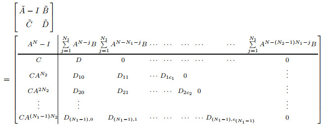
A4: The matrix
is of full row rank, where
and are quotient and remainder of , respectively (, )
A5: is detectable.
A6: Assume the preview length of the reference signal is , that is, at each time , the future values, , , , , as well as the present and past values of the reference signal are available where , and is a non-negative integer.
The future values of the reference signal are assumed not to change beyond the , namely
A6 is the standard assumption of preview control theory. In fact, the previewable signals have a significant effect on the performance of the control system only for a certain time period according to the characteristic of the control system itself. So we can ignore the reference signal when it extends beyond the preview length. To make it convenient for constructing an augmented error system, we assume the reference signal is any constant beyond the preview length.
The difference between reference signal and output signal is defined as the error signal.
In this paper, we would like to design a controller that makes the output vector track the reference signal without static error. That is,
3 Derivation of the Augmented Error System
First, by using the discrete lifting technique, the preview control problem of the general dual-rate discrete-time system is converted into the preview control problem of a single-rate system. During the derivation, we obtain the state-space model for a dual-rate sampled-data system. Based on the lifting system, we construct an augmented error system. Then we design the preview controller for the augmented error system.
3.1 State-Space Model of the Lifting System
Next, the general dual-rate discrete-time system is converted into a single-rate augmented system by using the lifting technique in [
13,
21]. Meanwhile the state-space model of this lifting system is given.
According to A1 and the available input-output data , the lifting system is obtained by lifting the input vector and output vector. Then we obtain a single-rate system with an underlying frame period .
Define the lifted input vector and lifted output vector as
And notice the zero-order holder, .
On the basis of [
13], we derive the lifted state-space model as
where
and each element in matrix is given by assumption A4.
3.2 The Construction of the Error System
According to the usual practice of preview control theory, we need to introduce the error signal and the future reference signals into the state vector. In this paper, we use the first-order forward difference operator :
First, construct the vector
Then we obtain the error vector:
From the second equation of (4), we get
Using on both sides of (7) and noticing that , we have
Then using on both sides of the first equation of (4), we have
Combining (8) and (9), we have
Letting
we have
The augmented error system (11) is the final system we needed.
In order to obtain a good transient response, we introduce the quadratic performance index of the augmented error system (11) as follows:
where , is a positive definite matrix, and is a positive definite matrix.
Now the preview control problem for system (1) with a dual-rate sampling setting is transformed into an optimal control problem for the augmented error system (11) minimizing the performance index (12). Noticing the error system (11), the reference signal vector is , which is previewable, that is, at any time , , , , are known, and
4 Design of a Preview Controller
Next we design the preview controller for the augmented error system (11). By using the results of preview control theory in [
1,
3], we know: If
is stabilizable and
is detectable, the optimal control input of system (11) minimizing the performance index (12) is given by
where
and is the unique symmetric semi-positive definite solution of the algebraic Riccati equation
Then we decompose and as follows:
Substituting and into (13), thus (13) can be written as
(19) can be written as
Noticing
we decompose into
So (20) can be written as
That is,
and
Based on the above derivation and the optimal control theory, we obtain the following theorem.
Theorem 1 If is stabilisable and is detectable, the optimal control input of system is
and
where the matrices and are determined by and , and the Riccati equation must be have the solution.
Noticing the last item of the optimal control input in Theorem 1, is the preview feedforward compensation item.
5 The Conditions of Controller Existence
Note that the conditions of controller existence are is stabilisable and is detectable in Theorem 1. In this section, some theorems are given by using Lemma 1 (PBH test), Lemma 2 and the relevant parameters of original system (1).
First, we see the stabilizability of .
Lemma 3 is stabilizable if and only if is stabilizable and the matrix is of full row rank.
Proof According to the PBH rank test in Lemma 1, we need to find a necessary and sufficient condition such that the matrix is of full row rank, where is any complex number and . We derive
Next we discuss this problem from two aspects.
If , is an invertible matrix. According to the properties of matrix rank, the matrix is of full row rank if and only if is of full row rank.
If , substituting into (23) we obtain the matrix We can see the matrix is of full row rank if and only if the matrix is of full row rank. That is, the matrix
(24)
is of full row rank. In conclusion, Lemma 3 is established.
Lemma 4 is stabilizable if and only if is stabilizable and , where is any eigenvalue of and .
Proof Use Lemma 2 to prove this lemma, noticing that
where .
We first prove the sufficiency of this lemma. From Lemma 2, if is stabilizable, for all and such that and , where is any eigenvalue of , is the corresponding left eigenvector and is the conjugate transposition of . We need to prove that is stabilizable, that is, for all and such that and , , where is any eigenvalue of and is the corresponding left eigenvector.
First, based on our knowledge of eigenvalue and eigenvector, the eigenvalue of must satisfy and , where and is any eigenvalue and . Furthermore, we can take as the corresponding left eigenvector of .
Second, from we can derive
So we have
On the other hand,
Because of , we have . Applying Lemma 2 again, sufficiency is proved.
Next, by using reduction to absurdity, the necessity of this lemma can be proved. We assume is stabilizable. If the conclusion is not established, that is, is not stabilizable or for some eigenvalue of and and noticing the eigenvalue of and the corresponding left eigenvector , we have
where is any eigenvalue of and . We still take as the corresponding left eigenvector of .
If is not stabilizable, then we have
So we get from (26), this contradicts the stabilizability of . Similarly, if for some eigenvalue of , we derive from (26) and this contradicts the stabilizability of . Thus, necessity is proved.
Therefore, according to Lemmas 3 and 4 we have
Theorem 2 is stabilizable if and only if is stabilizable and is any eigenvalue of and and the matrix by is of full row rank.
Theorem 2 shows that is stabilizable if and only if A3 and A4 hold. And the condition is both sufficient and necessary and these conditions guarantee the existence of the state feedback in Theorem 1.
Then, we examine the detectabiliy of .
Lemma 5 is detectable if and only if is detectable.
Proof Using the PBH rank test in Lemma 1, we have
Because of , is an invertible matrix. So is of full column rank if and only if is of full column rank. Applying the PBH rank test again, this lemma is established.
Lemma 6 is detectable if and only if is detectable.
Noticing
Letting , we have
Then
is detectable if and only if
is detectable by using the result in [
17]. So this lemma is proved.
Lemma 7 is detectable if and only if is detectable.
Proof Similar to the proof of Lemma 4, we first prove the sufficiency of this lemma. From Lemma 2, if is detectable, for all and such that and , , where is any eigenvalue of and is the corresponding right eigenvector. To prove that is detectable that for all and such that and , , where is any eigenvalue of and is the corresponding right eigenvector.
Based on our knowledge of eigenvalue and eigenvector, the eigenvalue of must satisfy and , where is any eigenvalue of and . Furthermore, we can take as the corresponding right eigenvector of .
Second, from we can derive So On the other hand, Using Lemma 2, we know that is detectable. Thus, sufficiency is proved.
Next, by using reduction to absurdity, the necessity of this lemma is proved. We assume is detectable. If the conclusion is not established, that is, is not detectable, and noticing the eigenvalue of and the corresponding right eigenvector , we have
where is any eigenvalue of and . We still take as the corresponding right eigenvector of .
If the conclusion is not established, that is, is not detectable, then we have
Obviously, this contradicts the detectability of . So we complete the proof.
Combining Lemma 5, Lemma 6 and Lemma 7, we obtain
Theorem 3 is detectable if and only if is detectable holds.
Notice that this is a sufficient and necessary condition, and it ensures that the Riccati equation (17) has a unique symmetric semi-positive definite solution.
According to the discussion of this section, Theorems 2 and 3 make the conditions in Theorem 1 can be satisfied and the Riccati equation (17) must have a unique semi-positive solution. Thus, the designed controller in Theorem 1 can be achieved.
6 Numerical Example
In this section, a numerical example is provided to demonstrate the effectiveness of the preview controller with a dual-rate setting.
Consider a linear discrete-time system
In comparison with system (1), the coefficient matrices are as follows:
Let and , that is, the output vector can only be measured at and the input vector can be input only at . Let the initial conditions be . In addition, take the weight matrices , .
Through verification, the system satisfies all the basic assumptions. According to Theorem 4, we perform Matlab simulation results for two kinds of reference signals as follows.
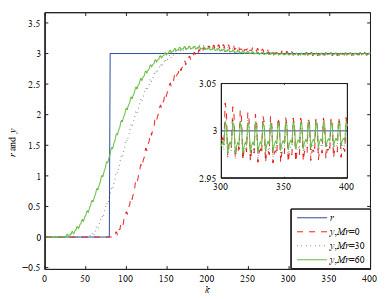
1)
The output response of the closed-loop system for System (27) is shown in Figure 1. And the subgraph shows a local enlarged simulation result. Under three situations (i.e., the preview lengths of the reference signal are , , and no preview (namely )), we can obviously see that the output can track the reference signal accurately. And we note that the preview action makes the tracking speed faster and reduces the error significantly. In addition, the output response curves show small oscillations, which are a feature of multirate systems.
Figure 1 The output response of the closed-loop system to reference signal (28) |
Full size|PPT slide
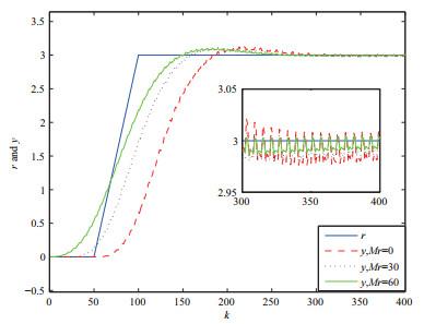
2)
The output response of the closed-loop system for System (27) is shown in Figure 2. And the subgraph shows a local enlarged simulation result. By comparing this with the output responses under different preview lengths, we observe that the preview action improves performance significantly.
Figure 2 The output response of the closed-loop system to reference signal (29) |
Full size|PPT slide
7 Conclusion
In this paper, the preview control problem based on the theory of multirate control is proposed for a type of discrete-time system with a dual-rate setting. First, adopting the discrete lifting technique, the general dual-rate discrete-time system is converted into a single-rate augmented system. And the lifted state-space model is obtained. Then we derive the augmented error system with a previewable reference signal by introducing a first-order difference operator. Finally, the optimal preview controller is designed by applying the results of preview control. In the meantime, the existence conditions of the preview controller are discussed in detail. The numerical simulations are presented to illustrate the effectiveness of the controller in this paper.
This paper extends the application of preview control in multirate systems. And its methods and conclusions can be further extended to discrete-time uncertain systems or discrete-time descriptor systems in subsequent research.
{{custom_sec.title}}
{{custom_sec.title}}
{{custom_sec.content}}
 PDF(239 KB)

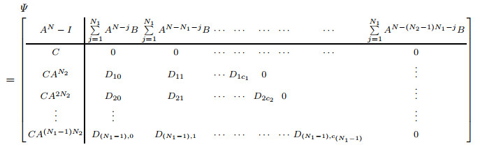
 Figure 1 The output response of the closed-loop system to reference signal (28)


