 PDF(775 KB)

A Metaheuristic Approach to Optimize European Call Function with Boundary Conditions
Najeeb Alam KHAN, Oyoon Abdul RAZZAQ, Tooba HAMEED
Journal of Systems Science and Information ›› 2018, Vol. 6 ›› Issue (3) : 260-268.
PDF(775 KB)
PDF(775 KB)
A Metaheuristic Approach to Optimize European Call Function with Boundary Conditions
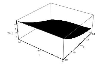
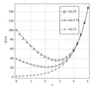
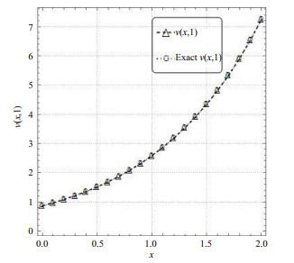
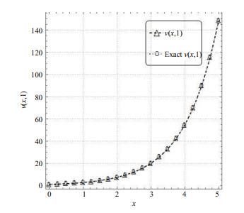
The purpose of this paper is to investigate the pricing European call option valuation problems under the exercise price, maturity, risk-free interest rate, and the volatility function. An advance methodology, Chebyshev simulated annealing neural network (ChSANN), is enforced for the Black-Scholes (B-S) model with boundary conditions. Our scheme is stable and easy to implement on B-S equation, for arbitrary volatility and arbitrary interest rate values. Also, the comparative results demonstrate that the attained approximate solutions are converging towards the exact solution. The graphical results show that the increasing flow of the European call option as the exponential increase takes place in assets. The presented algorithm can be further applied to other financial models with certain boundary conditions. The algorithm of the method shows that the approach can also be easily employed on time-fractional B-S equation.
neural network / numerical approximation / Chebyshev polynomials {{custom_keyword}} /
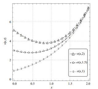
Figure 3 Flow patterns of |
Table 1 Global optimum mean square errors |
| 3 | 2.197 |
| 4 | 3.898 |
| 5 | 3.095 |
| 1 |
{{custom_citation.content}}
{{custom_citation.annotation}}
|
| 2 |
{{custom_citation.content}}
{{custom_citation.annotation}}
|
| 3 |
{{custom_citation.content}}
{{custom_citation.annotation}}
|
| 4 |
{{custom_citation.content}}
{{custom_citation.annotation}}
|
| 5 |
{{custom_citation.content}}
{{custom_citation.annotation}}
|
| 6 |
{{custom_citation.content}}
{{custom_citation.annotation}}
|
| 7 |
{{custom_citation.content}}
{{custom_citation.annotation}}
|
| 8 |
{{custom_citation.content}}
{{custom_citation.annotation}}
|
| 9 |
{{custom_citation.content}}
{{custom_citation.annotation}}
|
| 10 |
{{custom_citation.content}}
{{custom_citation.annotation}}
|
| 11 |
Khan N A, Shaik A, Sultan F, et al. Numerical simulation using artificial neural network on fractional differential equations. Numerical Simulation-From Brain Imaging to Turbulent Flow, InTech, doi: 10.5772/64151(2016).
{{custom_citation.content}}
{{custom_citation.annotation}}
|
| 12 |
{{custom_citation.content}}
{{custom_citation.annotation}}
|
| 13 |
{{custom_citation.content}}
{{custom_citation.annotation}}
|
| 14 |
{{custom_citation.content}}
{{custom_citation.annotation}}
|
| 15 |
{{custom_citation.content}}
{{custom_citation.annotation}}
|
| 16 |
{{custom_citation.content}}
{{custom_citation.annotation}}
|
| 17 |
{{custom_citation.content}}
{{custom_citation.annotation}}
|
| 18 |
{{custom_citation.content}}
{{custom_citation.annotation}}
|
| 19 |
{{custom_citation.content}}
{{custom_citation.annotation}}
|
| 20 |
{{custom_citation.content}}
{{custom_citation.annotation}}
|
| {{custom_ref.label}} |
{{custom_citation.content}}
{{custom_citation.annotation}}
|
PDF(775 KB)
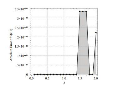
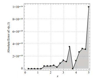
 Figure 1 Approximations of Figure 2 Approximations of Figure 3 Flow patterns of Figure 4 Flow patterns of Figure 5 Exact versus approximated solutions of Figure 6 Exact versus approximated solutions of Figure 7 Absolute error for Figure 8 Absolute error for
  Table 1 Global optimum mean square errors
 /
| 〈 |
|
〉 |


