Headings of UCAV Based on Nash Equilibrium

Li DAI; Zheng XIE

doi:10.21078/JSSI-2018-269-08

PDF(209 KB)

Journal of Systems Science and Information ›› 2018, Vol. 6 ›› Issue (3) : 269-276. DOI: 10.21078/JSSI-2018-269-08

Headings of UCAV Based on Nash Equilibrium

Author information +

History +

Abstract

Given n vertices in a plane and UCAV going through each vertex once and only once and then coming back, the objective is to find the direction (heading) of motion in each vertex to minimize the smooth path of bounded curvature. This paper studies the headings of UCAV. First, the optimal headings for two vertices were given. On this basis, an n-player two-strategy game theoretic model was established. In addition, in order to obtain the mixed Nash equilibrium efficiently, n linear equations were set up. The simulation results demonstrated that the headings given in this paper are effective.

Key words

UCAV / Dubins path / headings / Nash equilibrium / game theory

Cite this article

EndNote

Ris (Procite)

Bibtex

Download Citations

Li DAI , Zheng XIE. Headings of UCAV Based on Nash Equilibrium. Journal of Systems Science and Information, 2018, 6(3): 269-276 https://doi.org/10.21078/JSSI-2018-269-08

1 Introduction

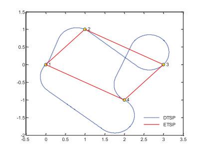
The trajectory of machines like UCAV (unmanned combat aircraft vehicles) or Robots is constrained by their kinematics. A suitable and useful mathematical model is DTSP (Dubins traveling salesman problem). Let

P = {p_{1}, p_{2}, \dots, p_{n}}

be a set of

n

vertices in a plane. The well-known TSP is to find the shortest tour (closed path) visiting every vertex once and only once. Depending on the definition of the distance between any pair of

n

vertices, TSP can be divided into two branches. One is the Euclidean traveling salesman problem (ETSP), in which the distance is defined as the Euclidean distance. The other is the Dubins traveling salesman problem (DTSP), in which the distance is defined as the Dubins distance. See Figure 1: The red line is the tour of ETSP, and the blue dotted line is the DTSP. DTSP differs from ETSP with respect to the constraint on the curvature of the tour; that is, the tour of the DTSP is smooth enough that the tour curvature is limited by

1 / ρ

, where

ρ

is the minimal turning radius.

Figure 1 ETSP and DTSP

Full size|PPT slide

It is well known that the ETSP is NP-complete^{[1, 2]} and that the DTSP is also NP-complete^[3].

Let ETSP

(P)

denote the length of the shortest tour of the ETSP over

P

. Correspondingly, let DTSP

_{ρ} (P)

denote the length of the shortest Dubins tour of the DTSP over

P

with the minimal turning radius

ρ

. Note that both ETSP

(P)

and DTSP

_{ρ} (P)

are in connection with the visiting order, and the optimal ETSP ordering of

P

might be quite different with the optimal DTSP ordering. So, we denote LETSP

_{(i_{1}, i_{2}, \dots, i_{n})} (P)

as the Euclidean distance, and LDTSP

_{(i_{1}, i_{2}, \dots, i_{n}), ρ} (P)

as the Dubins distance over

P

with the visiting order

(i_{1}, i_{2}, \dots, i_{n})

. Without confusion, they are abbreviated as LETSP

(P)

and LDTSP

_{ρ} (P)

If the visiting order

(i_{1}, i_{2}, \dots, i_{n})

is given, then LETSP

(P)

can be calculated as

L E T S P (P) = | p_{i_{1}} p_{i_{2}} | + | p_{i_{2}} p_{i_{3}} | + \dots + | p_{i_{n - 1}} p_{i_{n}} | + | p_{i_{n}} p_{i_{1}} |,

but the LDTSP

_{ρ} (P)

is still not easy to calculate because of unknown optimal headings. Let LDTSP

_{ρ, θ} (P)

be the Dubins distance with the visiting order

(i_{1}, i_{2} \dots, i_{n})

and the headings

θ = (θ_{i_{1}}, θ_{i_{2}}, \dots, θ_{i_{n}})

are given. Obviously,

{LDTSP}_{ρ, θ} (P) = \sum_{k = 1}^{n} {LD}_{ρ, (θ_{i_{k}}, θ_{i_{k + 1}})} (p_{i_{k}}, p_{i_{k + 1}}),

where

{LD}_{ρ, (θ_{i_{k}}, θ_{i_{k + 1}})} (p_{i_{k}}, p_{i_{k + 1}})

is the Dubins distance between

p_{i_{k}}

and

p_{i_{k + 1}}

, and

θ_{i_{n + 1}} = θ_{i_{1}}

p_{i_{n + 1}} = p_{i_{1}}

To calculate

{LD}_{ρ, (θ_{i_{k}}, θ_{i_{k + 1}})} (p_{i_{k}}, p_{i_{k + 1}})

, we can use the famous results given by Dubins in 1957^[4]. Dubins gave a sufficient set of paths (the Dubins set) that always contains the shortest path between any two vertices with given headings. The famous Dubins set is

{L S L, R S R, L S R, R S L, R L R, L R L},

which includes six admissible paths, where

L

and

R

are arcs of the minimal allowed turning radius

ρ

turning left or turning right, respectively, and

S

is a segment. In 2001, Shkel and Lumelsky considered the logical classification scheme, which allows one to extract the shortest path from the Dubins set directly, without explicitly calculating the candidate paths for the 'long path case'^[5]. In [5], the initial vertex is

(0, 0; α)

, the terminal vertex is

(d, 0; β)

and the radius

ρ = 1

For DTSP, there are

n

vertices and cases with any initial and terminal vertices need to be considered. In 2015, Dai and Xie provided the formula to directly calculate the length of the Dubins distance with any initial vertex

(x_{0}, y_{0}; α)

, terminal vertex

(x_{1}, y_{1}; β)

and minimal turning radius

ρ > 0

^[6].

Obviously, there are two key problems in the DTSP: Determining the optimal visiting order

(i_{1}, i_{2}, \dots, i_{n})

and the optimal headings

(θ_{i_{1}}, θ_{i_{2}}, \dots, θ_{i_{n}})

. The majority of papers focus on the optimal visiting order rather than the optimal headings. Savla, et al.^[7] presented a way to calculate the headings of each vertex, and based on this type of heading, they provided an algorithm called Alternating Algorithm (AA), and they proved that the upper bound of DTSP is

{DTSP}_{ρ} (P) \leq ETSP (P) + κ ⌈ \frac{n}{2} ⌉ π ρ,

(1)

where

κ \in [2.657, 2.658]

. In 2013, Kim and Cheong proved in their paper^[8] that

κ = \frac{7}{3}

We focus on determining the optimal headings. Note that the fitness of one vertex's head depends on both its own and the neighbor's as well. So, we modeled this problem based on Game Theory, which has received an increasing amount of attention as a promising technique for formulating action strategies for agents in complex situations. The priority of Game Theory in solving control and decision-making problems has been shown in many studies^[9-15].

Finding the Nash Equilibrium in an

n

-player

(n \geq 3)

game has been proved to be PPAD-complete^{[16, 17]}. So, the problem of computing Nash Equilibria in games is computationally extremely difficult, if not impossible. But, for a two-player game, it is much easier to solve.

The main contribution of this paper is the development of a game theoretic approach to the DTSP. The headings of vertices are handled from a game theoretic perspective and obtained efficiently by solving the mixed Nash equilibrium of an

n

-player two-strategy game.

The remainder of the paper is organized as follows: Section 2 is the main body of this paper, it describes the Game Theory model for determining better headings and introduces the theory of the Nash Equilibrium. Section 3 concludes our conclusions.

2 Game Theory model

Let

p_{1}, p_{2}, \dots, p_{n}

n

vertices in a plane. Without loss of generality, let the optimal visiting order be

p_{1} \to p_{2} \to \dots \to p_{n} \to p_{1}

. So, there are

n

players

p_{1}, p_{2}, \dots, p_{n}

in the game. Each player

p_{i}

choose it's heading

θ_{i} \in [0, 2 π] (i = 1, 2, \dots, n)

. The heading

θ_{i}

is seen as a pure strategy in the game. We defined the payoff of player

p_{i}

as the Dubins distance

{LD}_{ρ, (θ_{i}, θ_{i + 1})} (p_{i}, p_{i + 1})

between

p_{i}

and

p_{i + 1}

for all

i \in {1, 2, \dots, n}

(where

p_{n + 1} = p_{1}

The Dubins distance changes greatly with the headings. So, which heading

θ_{i}

to choose is the key problem. When

θ_{i}

ranges from

0

2 π

, there is an infinitely pure strategy for each vertex

p_{i}

. The problem is difficult to solve because the Dubins distance is not a continuous function.

2.1 Pure Strategies and Payoffs

In this section, we consider the length of the optimal Dubins tour with two vertices. Let

A (0, 0)

be the initial vertex and

B (d, 0)

be the terminal vertex. DTSP

_{ρ} (A, B)

denotes the length of the optimal Dubins tour. We have the following Proposition 1, which suggests that there are only two pure strategies that need to be considered for each vertex.

Proposition 1 For two vertices, $A (0, 0)$ and $B (d, 0)$ ,

(ⅰ) If

d \geq 2 ρ

{DTSP}_{ρ} (A, B) = 2 π ρ + 2 (d - 2 ρ)

(ⅱ) If

d \leq 2 ρ

{DTSP}_{ρ} (A, B) = 2 π ρ

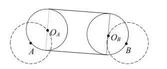
Proof (ⅰ) Based on the Dubins result in 1957, the minimum length between any two vertices must lie in the following Dubins set

{R S R, R S L, L S R, L S L, R L R, L R L}

. By noting that these six types of Dubins paths all start and end with an arc with radius

ρ

, let

A

and

B

be the center and

ρ

be the radius; we draw two circles

⨀ A

and

⨀ B

. See the circles with dotted lines in Figure 2.

Figure 2 The Dubins tour for two vertices with $ρ \leq d / 2$

Full size|PPT slide

It can be observed that given any arc with radius

ρ

and which

A

lies on, its center must lie in the circle

⨀ A

. This is also the case with

B

. Then, the Dubins tour depends on the position of the center. Without loss of generality, we set the centers as

O_{A}

and

O_{B}

. See Figure 2. The length of the Dubins tour is

2 π ρ + 2 O_{A} O_{B}

. And the minimum length of

O_{A} O_{B}

d - 2 ρ

(ⅱ) If

d \leq 2 ρ

⨀ A

and

⨀ B

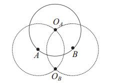
must intersect at two places. See Figure 3. Let

⨀ A

and

⨀ B

intersect at

O_{A}

and

O_{B}

. Then, both

A

and

B

lie in the circle

⨀ O_{A}

(or

⨀ O_{B}

) with radius

ρ

. So the minimum length of the Dubins tour must not be larger than

2 π ρ

Figure 3 The Dubins tour for two vertices with $ρ \geq d / 2$

Full size|PPT slide

On the other hand, when we travel from the initial vertex

A

with the minimal turning radius

ρ

and come back to

A

, the minimal length needed is

2 π ρ

regardless of whether

B

is visited.

Proposition 1 gives the optimal Dubins tour for two vertices, and it also tells us the optimal headings

θ_{A}

of initial vertex

A

and

θ_{B}

of the terminal vertex

B

, that is,

θ_{A} = {\begin{cases} π / 2, & ρ \leq \frac{d}{2}, \\ π / 2 + \arccos \frac{d}{2 ρ}, & ρ \geq \frac{d}{2} . \end{cases} θ_{B} = {\begin{cases} - π / 2, & ρ \leq \frac{d}{2}, \\ π + \arcsin \frac{d}{2 ρ}, & ρ \geq \frac{d}{2} . \end{cases}

(2)

Further, for any initial vertex

A (x_{A}, y_{A})

and terminal vertex

B (x_{B}, y_{B})

, let

θ_{A B}

be the angle of vector

\vec{A B}

. Ihe optimal headings

{\hat{θ}}_{A}

and

{\hat{θ}}_{B}

would be

{\hat{θ}}_{A} = θ_{A} + θ_{A B}, {\hat{θ}}_{B} = θ_{B} + θ_{A B} .

(3)

There are

n

players

p_{1}, p_{2}, \dots, p_{n}

in the game. Let

S_{i}

be the strategy set of

p_{i}

then, by Proposition 1, we have

S_{i} = {θ_{i 1}, θ_{i 2}},

where

θ_{i 1}

and

θ_{i 2}

are both determined by (3), and

θ_{i 1}

is the heading of

p_{i}

when

p_{i - 1}

is the initial vertex and

p_{i}

is the terminal vertex,

θ_{i 2}

is determined by

p_{i}

is the initial vertex and

p_{i + 1}

is the terminal vertex.

The payoff of

p_{i}

is defined as

u_{i} = {LD}_{ρ, (θ_{i}, θ_{i + 1})} (p_{i}, p_{i + 1}) + {LD}_{ρ, (θ_{i - 1}, θ_{i})} (p_{i - 1}, p_{i}), i = 1, 2, \dots, n .

(4)

From a game theory point of view, each vertex tries to minimize its own payoff by calculating a pure strategy Nash equilibrium or a mixed Nash Equilibrium. In this way, we get an

n

-players two strategies game.

2.2 Nash Equilibrium

Let

(θ_{1 i_{1}}, θ_{2 i_{2}}, \dots, θ_{n i_{n}})

be a pure strategy Nash equilibrium, Note that each vertex tries to minimize its own payoff for the length of DTSP, so we have

u_{j} (θ_{j i_{j}}, θ_{- j}) \leq u_{j} (θ_{j i_{k}}, θ_{- j}), \forall θ_{j i_{k}} \in S_{j}, j \in {1, 2, \dots, n} .

(5)

If player

p_{i}

has a pure strategy in a Nash equilibrium, from (5), we need to make

2^{n - 1}

comparisons for each

u_{i}

If player

p_{i}

does not have a pure strategy, we need to consider its mixed strategy.

Let

x^{i} = (x_{i}, 1 - x_{i})

be the mixed strategy of player

p_{i}

, that is, the heading

θ_{i 1}

of vertex

p_{i}

is selected with a probability of

x_{i}

and

θ_{i 2}

is selected with a probability of

1 - x_{i} (i = 1, 2, \dots, n)

, where

x_{i} \in (0, 1)

. Let

x = (x^{1}, x^{2}, \dots, x^{n})

be the mixed Nash equilibrium. We have the following proposition 2.

Proposition 2 Let $x = (x^{1}, x^{2}, \dots, x^{n})$ be the mixed Nash equilibrium, where $x^{i} = (x_{i}, 1 - x_{i})$ and $x_{i} \neq 0 (i = 1, 2, \dots, n)$ , then, for any $i \in {1, 2, \dots, n}$ ,

\begin{array}{rcl} [{L D}_{ρ, (θ_{i - 1, 1}, θ_{i, 2})} (p_{i - 1}, p_{i}) - {L D}_{ρ, (θ_{i - 1, 2}, θ_{i, 2})} (p_{i - 1}, p_{i}) \\ - {L D}_{ρ, (θ_{i - 1, 1}, θ_{i, 1})} (p_{i - 1}, p_{i}) + {L D}_{ρ, (θ_{i - 1, 2}, θ_{i, 1})} (p_{i - 1}, p_{i})] \cdot x_{i - 1} \\ + [{L D}_{ρ, (θ_{i, 2}, θ_{i + 1, 1})} (p_{i}, p_{i + 1}) - {L D}_{ρ, (θ_{i, 2}, θ_{i + 1, 2})} (p_{i}, p_{i + 1}) \\ - {L D}_{ρ, (θ_{i, 1}, θ_{i + 1, 1})} (p_{i}, p_{i + 1}) + {L D}_{ρ, (θ_{i, 1}, θ_{i + 1, 2})} (p_{i}, p_{i + 1})] \cdot x_{i + 1} \\ + [{L D}_{ρ, (θ_{i - 1, 2}, θ_{i, 2})} (p_{i - 1}, p_{i}) + {L D}_{ρ, (θ_{i, 2}, θ_{i + 1, 2})} (p_{i}, p_{i + 1}) \\ - {L D}_{ρ, (θ_{i - 1, 2}, θ_{i, 1})} (p_{i - 1}, p_{i}) - {L D}_{ρ, (θ_{i, 1}, θ_{i + 1, 2})} (p_{i}, p_{i + 1})] = 0. \end{array}

Proof Since

x

is a mixed Nash equilibrium, we have

x_{i} \cdot (E_{i} (x) - E_{i} (θ_{i 1}, x_{- i})) = 0, (1 - x_{i}) \cdot (E_{i} (x) - E_{i} (θ_{i 2}, x_{- i})) = 0, \forall i \in {1, 2, \dots, n} .

Because of

x_{i} \neq 0

, then

E_{i} (θ_{i 1}, x_{- i}) = E_{i} (x) = E_{i} (θ_{i 2}, x_{- i}) .

By the definition of expected payoff,

\begin{array}{l} E_{i} (θ, x_{- i}) = ({L D}_{ρ, (θ_{i - 1, 1}, θ)} (p_{i - 1}, p_{i}) + {L D}_{ρ, (θ, θ_{i + 1, 1})} (p_{i}, p_{i + 1})) \cdot x_{i - 1} \cdot x_{i + 1} \\ + ({L D}_{ρ, (θ_{i - 1, 1}, θ)} (p_{i - 1}, p_{i}) + {L D}_{ρ, (θ, θ_{i + 1, 2})} (p_{i}, p_{i + 1})) \cdot x_{i - 1} \cdot (1 - x_{i + 1}) \\ + ({L D}_{ρ, (θ_{i - 1, 2}, θ)} (p_{i - 1}, p_{i}) + {L D}_{ρ, (θ, θ_{i + 1, 1})} (p_{i}, p_{i + 1})) \cdot (1 - x_{i - 1}) \cdot x_{i + 1} \\ + ({L D}_{ρ, (θ_{i - 1, 2}, θ)} (p_{i - 1}, p_{i}) + {L D}_{ρ, (θ, θ_{i + 1, 2})} (p_{i}, p_{i + 1})) \cdot (1 - x_{i - 1}) \cdot (1 - x_{i + 1}) \\ = {L D}_{ρ, (θ_{i - 1, 1}, θ)} (p_{i - 1}, p_{i}) \cdot x_{i - 1} + {L D}_{ρ, (θ_{i - 1, 2}, θ)} (p_{i - 1}, p_{i}) \cdot (1 - x_{i - 1}) \\ + {L D}_{ρ, (θ, θ_{i + 1, 1})} (p_{i}, p_{i + 1}) \cdot x_{i + 1} + {L D}_{ρ, (θ, θ_{i + 1, 2})} (p_{i}, p_{i + 1}) \cdot (1 - x_{i + 1}) . \\ = [{L D}_{ρ, (θ_{i - 1, 1}, θ)} (p_{i - 1}, p_{i}) - {L D}_{ρ, (θ_{i - 1, 2}, θ)} (p_{i - 1}, p_{i})] \cdot x_{i - 1} \\ + [{L D}_{ρ, (θ, θ_{i + 1, 1})} (p_{i}, p_{i + 1}) - {L D}_{ρ, (θ, θ_{i + 1, 2})} (p_{i}, p_{i + 1})] \cdot x_{i + 1} \\ + [{L D}_{ρ, (θ_{i - 1, 2}, θ)} (p_{i - 1}, p_{i}) + {L D}_{ρ, (θ, θ_{i + 1, 2})} (p_{i}, p_{i + 1})] . \end{array}

then by

E_{i} (θ_{i 1}, x_{- i}) = E_{i} (θ_{i 2}, x_{- i}),

we have

\begin{array}{l} [{L D}_{ρ, (θ_{i - 1, 1}, θ_{i, 2})} (p_{i - 1}, p_{i}) - {L D}_{ρ, (θ_{i - 1, 2}, θ_{i, 2})} (p_{i - 1}, p_{i})] \cdot x_{i - 1} \\ + [{L D}_{ρ, (θ_{i, 2}, θ_{i + 1, 1})} (p_{i}, p_{i + 1}) - {L D}_{ρ, (θ_{i, 2}, θ_{i + 1, 2})} (p_{i}, p_{i + 1})] \cdot x_{i + 1} \\ + [{L D}_{ρ, (θ_{i - 1, 2}, θ_{i, 2})} (p_{i - 1}, p_{i}) + {L D}_{ρ, (θ_{i, 2}, θ_{i + 1, 2})} (p_{i}, p_{i + 1})] \\ = [{L D}_{ρ, (θ_{i - 1, 1}, θ_{i, 1})} (p_{i - 1}, p_{i}) - {L D}_{ρ, (θ_{i - 1, 2}, θ_{i, 1})} (p_{i - 1}, p_{i})] \cdot x_{i - 1} \\ + [{L D}_{ρ, (θ_{i, 1}, θ_{i + 1, 1})} (p_{i}, p_{i + 1}) - {L D}_{ρ, (θ_{i, 1}, θ_{i + 1, 2})} (p_{i}, p_{i + 1})] \cdot x_{i + 1} \\ + [{L D}_{ρ, (θ_{i - 1, 2}, θ_{i, 1})} (p_{i - 1}, p_{i}) + {L D}_{ρ, (θ_{i, 1}, θ_{i + 1, 2})} (p_{i}, p_{i + 1})] . \end{array}

That is,

\begin{array}{l} [{L D}_{ρ, (θ_{i - 1, 1}, θ_{i, 2})} (p_{i - 1}, p_{i}) - {L D}_{ρ, (θ_{i - 1, 2}, θ_{i, 2})} (p_{i - 1}, p_{i}) \\ - {L D}_{ρ, (θ_{i - 1, 1}, θ_{i, 1})} (p_{i - 1}, p_{i}) + {L D}_{ρ, (θ_{i - 1, 2}, θ_{i, 1})} (p_{i - 1}, p_{i})] \cdot x_{i - 1} \\ + [{L D}_{ρ, (θ_{i, 2}, θ_{i + 1, 1})} (p_{i}, p_{i + 1}) - {L D}_{ρ, (θ_{i, 2}, θ_{i + 1, 2})} (p_{i}, p_{i + 1}) \\ - {L D}_{ρ, (θ_{i, 1}, θ_{i + 1, 1})} (p_{i}, p_{i + 1}) + {L D}_{ρ, (θ_{i, 1}, θ_{i + 1, 2})} (p_{i}, p_{i + 1})] \cdot x_{i + 1} \\ + [{L D}_{ρ, (θ_{i - 1, 2}, θ_{i, 2})} (p_{i - 1}, p_{i}) + {L D}_{ρ, (θ_{i, 2}, θ_{i + 1, 2})} (p_{i}, p_{i + 1}) \\ - {L D}_{ρ, (θ_{i - 1, 2}, θ_{i, 1})} (p_{i - 1}, p_{i}) - {L D}_{ρ, (θ_{i, 1}, θ_{i + 1, 2})} (p_{i}, p_{i + 1})] = 0. \end{array}

By Proposition 2, we will get

n

linear equations. The solution of the equations will be the mixed Nash equilibrium.

Above all, we set up a Game Theory model for headings of DTSP. The vertice

p_{1}, p_{2}, \dots, p_{n}

are the players, and each player has two strategies given by (3), and the payoff defined as (

4

). For the Nash equilibrium, we first discuss whether it has a pure strategy Nash equilibrium. If it does not have a pure strategy for some players, we obtain its mixed strategy from Proposition 2 by solving linear equations.

2.3 An Example

Let

p_{1} (0, 0), p_{2} (1, 1), p_{3} (3, 0)

be three vertices in a plane and

ρ = 1

. By (3), we get the strategies

S_{i}

of each player

p_{i}

S_{1} = {3.1416, 1.5708}, S_{2} = {4.7124, 1.1071}, S_{3} = {4.2488, 4.7124} .

The payoffs are as follows:

\begin{array}{l} {LD}_{ρ, (θ_{11}, θ_{21})} (p_{1}, p_{2}) = 4.7124, {LD}_{ρ, (θ_{11}, θ_{22})} (p_{1}, p_{2}) = 6.7325, \\ {LD}_{ρ, (θ_{12}, θ_{21})} (p_{1}, p_{2}) = 5.7778, {LD}_{ρ, (θ_{12}, θ_{22})} (p_{1}, p_{2}) = 7.6407, \\ {LD}_{ρ, (θ_{21}, θ_{31})} (p_{2}, p_{3}) = 8.2035, {LD}_{ρ, (θ_{21}, θ_{32})} (p_{2}, p_{3}) = 8.5193, \\ {LD}_{ρ, (θ_{22}, θ_{31})} (p_{2}, p_{3}) = 3.3776, {LD}_{ρ, (θ_{22}, θ_{32})} (p_{2}, p_{3}) = 3.2406, \\ {LD}_{ρ, (θ_{31}, θ_{11})} (p_{3}, p_{1}) = 3.2911, {LD}_{ρ, (θ_{31}, θ_{12})} (p_{3}, p_{1}) = 3.8706, \\ {LD}_{ρ, (θ_{32}, θ_{11})} (p_{3}, p_{1}) = 3.8578, {LD}_{ρ, (θ_{32}, θ_{12})} (p_{3}, p_{1}) = 4.1416 . \end{array}

By the formula of payoff (4), we have Table 1, and from this Table, we know that for all

i, j \in {1, 2}

\begin{array}{l} u_{1} (θ_{11}, θ_{2 i}, θ_{3 j}) < u_{1} (θ_{12}, θ_{2 i}, θ_{3 j}), \\ u_{2} (θ_{1 i}, θ_{21}, θ_{3 j}) > u_{2} (θ_{1 i}, θ_{22}, θ_{3 j}), \\ u_{3} (θ_{1 i}, θ_{2 j}, θ_{31}) < u_{3} (θ_{1 i}, θ_{2 j}, θ_{32}), \end{array}

Table 1 Payoff of the three players

	$u_{1}$	$u_{2}$	$u_{3}$
$θ_{11}, θ_{21}, θ_{31}$	8.0035	12.9159	11.4946
$θ_{11}, θ_{21}, θ_{32}$	8.5702	13.2317	12.3771
$θ_{11}, θ_{22}, θ_{31}$	10.0236	10.1101	6.6687
$θ_{11}, θ_{22}, θ_{32}$	10.5903	9.9731	7.0984
$θ_{12}, θ_{21}, θ_{31}$	9.6484	13.9813	12.0741
$θ_{12}, θ_{21}, θ_{32}$	9.9194	14.2971	12.6609
$θ_{12}, θ_{22}, θ_{31}$	11.5113	11.0183	7.2482
$θ_{12}, θ_{22}, θ_{32}$	11.7823	10.8813	7.3822

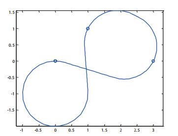
So, there exists a pure strategy Nash equilibrium

(θ_{11}, θ_{22}, θ_{31})

. The length of the DTSP is

{LDTSP}_{ρ} (P) = \frac{1}{2} (u_{1} (θ_{11}, θ_{22}, θ_{31}) + u_{2} (θ_{11}, θ_{22}, θ_{31}) + u_{3} (θ_{11}, θ_{22}, θ_{31})) = 13.4012 .

The tour curvature is given in Figure 4.

Figure 4 DTSP with heading given by a pure strategy Nash equilibrium

Full size|PPT slide

The length of ETSP is

ETSP (P) = | p_{1} p_{2} | + | p_{2} p_{3} | + | p_{3} p_{1} | = 6.6503

, and

ETSP (P) + \frac{7}{3} ⌈ \frac{n}{2} ⌉ π ρ \approx 21.3111 .

So, the length of DTSP with headings given by the Nash equilibrium is much smaller than the upper bound given by (1).

3 Conclusions

In this paper, we study the headings of the DTSP, which is widely used in the field, e.g., UCAV and Robots. It is important to note that we design the headings based on Game Theory. It is the Nash equilibrium that makes our headings quite different.

The simple example in Subsection 2.3 shows that the

n

-player two-strategy Game Theory model provides fairly good headings. In addition, the Nash equilibrium in this model is a pure strategy. The mixed Nash equilibrium can be easily obtained by solving the linear equations given in Proposition 2.

All vertices

p_{1}, p_{2}, \dots, p_{n}

are in a plane. So, how to determine the headings when the points are located in the three-dimensional space is worth further study. Since any three vertices in a three-dimensional space are coplanar, the presented results in this paper also give a new interesting insight into the three-dimensional DTSP problem.

References

Publishing order | Descend order by publishing year | Descend order by cited within

1	Papadimitriou C. The Euclidean traveling salesman problem is NP-complete. Theor. Comp. Sci., 1977, 4 (3): 237- 244. https://doi.org/10.1016/0304-3975(77)90012-3 Cited in this article [1]

2	Garey M R, Graham R L, Johnson D S. Some NP-complete geometric problems. Proc. 8th Annu. ACM Symp. Theory Comp., 1976, 10- 22. Cited in this article [1]

3	Ny J L, Feron E, Frazzoli E. On the Dubins traveling salesman problem. IEEE Transactions on Autonatic Control, 2012, 57, 265- 270. https://doi.org/10.1109/TAC.2011.2166311 Cited in this article [1]

4	Dubins L E. On curves of minimal length with a constraint on average curvature and with prescribed initial and terminal positions and Tangents. American Journal of Mathematics, 1957, 79, 497- 516. https://doi.org/10.2307/2372560 Cited in this article [1]

5	Shkel A M, Lumelsky V. Classification of the Dubins set. Robotics and Automonous Systems, 2001, 34, 179- 202. https://doi.org/10.1016/S0921-8890(00)00127-5 Cited in this article [2]

6	Dai L, Xie Z. On the length of dubins path with any initial and terminal configurations. Pure and Applied Mathematics Journal, 2015, 4, 248- 254. https://doi.org/10.11648/j.pamj.20150406.14 Cited in this article [1]

7	Savla K, Frazzoli E, Bullo F. Traveling salesman problems for the Dubins vehicle. IEEE Transections on Automatic Control, 2008, 53, 1378- 1391. https://doi.org/10.1109/TAC.2008.925814 Cited in this article [1]

8	Kim H S, Cheong O. The cost of bounded curvature. Computational Geometry: Theory and Applications, 2013, 46, 648- 672. https://doi.org/10.1016/j.comgeo.2012.10.008 Cited in this article [1]

9	Dixon W. Optimal adaptive sontrol and differential games by reinforcement learning principles. Journal of Guidance, Control, and Dynamics, 2014, 37 (3): 1048- 1049. https://doi.org/10.2514/1.G000173 Cited in this article [1]

10	Gu D. A game theory approach to target tracking in sensor networks. IEEE Transactions Systems, Man and Cybernetics, Part B: Cybernetices, 2011, 41 (1): 2- 13. https://doi.org/10.1109/TSMCB.2010.2040733

11	Duan H, Wei X, Dong Z. Multiple UCVAs cooperative air combat simulation platform based on PSO, ACO, and game theory. IEEE Aerospace and Electronic Systems Magazine, 2013, 28 (11): 12- 19. https://doi.org/10.1109/MAES.2013.6678487

12	Duan H, Pei L, Yuan Y X. A predator-prey particle swarm optimization approach to multiple UCAV air combat modeled by dynamic game theory. IEEE Journal of Automatica Sinica, 2015, 2 (1): 11- 18. https://doi.org/10.1109/JAS.2015.7032901

13	Wang M, Du Z, Duan H. Study on participant behavior game of electronic products reverse supply chain based on ECP. Journal of Systems Science and Information, 2017, 5 (5): 441- 434. https://syssci.cjoe.ac.cn/EN/10.21078/JSSI-2017-411-24

14	Wu J, Yang H, Cheng Y. Domino effect analysis, assessment and prevention in process industries. Journal of Systems Science and Information, 2015, 3 (6): 481- 498. https://doi.org/10.1515/JSSI-2015-0481

15	Dai Y, Gao Y. Real-time pricing decision based on leader-follower game smart grid. Journal of Systems Science and Information, 2015, 3 (6): 481- 498. https://doi.org/10.1515/JSSI-2015-0481 Cited in this article [1]

16	Porter R, Nudelman E, Shoham Y. Simple search methods for finding a Nash equilibrium. Games and Economic Behavior, 2008, 63 (2): 642- 662. https://doi.org/10.1016/j.geb.2006.03.015 Cited in this article [1]

17	Chen X, Deng X, Teng S H. Settling the complexity of computing two-player Nash equilibrium. Journal of the ACM, 2009, 56 (3): Article No.14. Cited in this article [1]

Funding

Research Programme of National University of Defense Technology(JC14-02-10)

PDF(209 KB)

186

Accesses

Citation

Detail

Sections

Recommended

Abstract
Key words
Cite this article
1 Introduction
Figure 1 ETSP and DTSP
2 Game Theory model
2.1 Pure Strategies and Payoffs
Figure 2 The Dubins tour for two vertices with $ρ \leq d / 2$
Figure 3 The Dubins tour for two vertices with $ρ \geq d / 2$
2.2 Nash Equilibrium
2.3 An Example
Table 1 Payoff of the three players
Figure 4 DTSP with heading given by a pure strategy Nash equilibrium
3 Conclusions
References
Funding

Received	Accepted	Published
2017-05-03	2017-12-07	2018-06-25
Issue Date
2018-06-25

Please choose a citation manager

Content to export

Abstract

Key words

Cite this article

1 Introduction

Figure 1 ETSP and DTSP

2 Game Theory model

2.1 Pure Strategies and Payoffs

Figure 2 The Dubins tour for two vertices with $ρ \leq d / 2$

Figure 3 The Dubins tour for two vertices with $ρ \geq d / 2$

2.2 Nash Equilibrium

2.3 An Example

Table 1 Payoff of the three players

Figure 4 DTSP with heading given by a pure strategy Nash equilibrium

3 Conclusions

{{custom_sec.title}}

{{custom_sec.title}}

References

{{custom_fnGroup.title_en}}

Footnotes

Funding

Share

模态框（Modal）标题

Please choose a citation manager

Content to export

Abstract

Key words

Cite this article

1 Introduction

Figure 1 ETSP and DTSP

2 Game Theory model

2.1 Pure Strategies and Payoffs

Figure 2 The Dubins tour for two vertices with ρ≤d/2

Figure 3 The Dubins tour for two vertices with ρ≥d/2

2.2 Nash Equilibrium

2.3 An Example

Table 1 Payoff of the three players

Figure 4 DTSP with heading given by a pure strategy Nash equilibrium

3 Conclusions

{{custom_sec.title}}

{{custom_sec.title}}

References

{{custom_fnGroup.title_en}}

Footnotes

Funding

Figure 2 The Dubins tour for two vertices with $ρ \leq d / 2$

Figure 3 The Dubins tour for two vertices with $ρ \geq d / 2$