1 Introductions
GPS (global positioning system) positioning is able to obtain receiver position by calculating the distance from satellite to receiver and satellite position
[1, 2], the distance that from satellite to receiver would be equal to the multiplication between propagation velocity and propagation time, thus, calculating the satellite position is a key element in GPS positioning. Given by global tracking station, GPS precise ephemeris can provide high precision and discrete satellite position
[3-6], but not apply satellite position at any observation time. Therefore, how to obtain the satellite position at any observation time is of significance problem in the study of GPS positioning. The interpolation method has advantages of simple process, high computational efficiency, which can get the epoch instantaneous satellite position. Interpolation is a matter of being composed of lots of known discrete variables and the corresponding dependent variable value, besides, being established polynomial function, which can be drawn the variable value at any discrete points. There are a variety of interpolation methods in resolving satellite position, this paper mainly studies Lagrange interpolation, Newton interpolation, Hermite interpolation method, Cubic spline interpolation method, Chebyshev fitting method. Apart from, the article describes the principle of several methods, analyses the calculation precision of each method and discusses advantages and disadvantages, finally, comes to the optimal interpolation method in satellite position solution.
2 Interpolation Method
2.1 Lagrange Interpolation
In the independent variable
,
has
points
, and its corresponding values are
separately
[7, 8]. Given an
in
, we are capable of getting the corresponding estimate of
. The basic formula is as follows:
Formula (1), denotes Lagrange interpolation polynomial; denotes numbers; denotes the function value of point ; stands for basic function, its formula is:
Formula (2), , separately stands for different time nodes; is to be inserted points; and are numbers. Given a in , then you will get a estimate of by means of Formula (1) and Formula (2). If there are two discrete points in , so Formula (1) is the linear interpolation function, if there are three discrete points , then Formula (1) is parabolic interpolation function, if there are points , thus Formula (1) is times polynomial function. During calculating satellite position, in a certain observation period, in order to obtain the satellite position at any epoch of the period, Formula (1) can be written as:
Formula (3)(5), expresses observation time of the interpolation node; expresses a basic function; , , respectively signify numbers corresponding satellite positions , in three directions; , , are separately satellites positions at the moment in three directions.
2.2 Newton Interpolation
Function
has
discrete points
in the independent variable
and its corresponding dependent variable values separately signify
, given a
in
, corresponding dependent variable value is
[9, 10]. The first step of this method is to find the value in the divided difference table, then
, correspondingly,
is:
In addition:
Formula (6) (7), indicates that numbers interpolation polynomial; represents function value of independent variable ; is arbitrary interpolation point; are independent variables; expresses divided difference of n orders.
A good characteristic of Newton interpolation method is that it never waste information in the divided difference table when we increases one discrete point for the independent variables, this algorithm are about to add the corresponding independent variables, the dependent variables and the difference to the divided difference table, which applied to Formula (6) can calculate function value of point to be inserted. Meanwhile, in the satellite position calculation, Formula (6) is derived as:
Formula (8)(10), are regarded as the observation time of independent variables; represents interpolation observation time; represents n orders difference at observation time ; , , respectively stand for the satellite position at time in three directions.
Though Formula (8), (9) and (10) can be calculated satellite position at any epoch.
2.3 Hermite Interpolation
, this method only consider that the function has uninterrupted features and has smooth features, taking a number of points in and the corresponding value to compose interpolation polynomial function whose function values are separately at the point .
Duing to function and satisfy:
Therefore both of them have a close degree. In the , , ( has numbers), there are known values, thus, is as follows:
Formula (11), denotes an independent variable; denotes a function whose times are less than . denote function coefficient.
Function consists of Formula (2):
Formula (12), denotes the satellite coordinates in three directions; stands for the first derivative value at each node; , composed of the basic function stands for times polynomial. We take advantage of coordinates at each node and the one order derivative value of each node in the polynomial function constructed by the method of 2.1 sections to calculate satellite position.
2.4 Cubic Spline Interpolation
The interval is divided into parts: . Given a point in and the dependent variable value , if there exits a polynomial contends the following three conditions, then is called the interpolation function at the point .
1) Interpolation condition:
Formula (13), represents a point in ; represents the known dependent variable value at the point ; represents the interpolation function value at the point .
2) Subsection condition: Within a cell interval, is a three algebraic polynomial:
Formula (14), is any point in ; stands for interpolation function; are polynomial coefficient.
3) Smooth condition: , that is to say, has continuous feature. Moreover, stands for the value of at point , stands for bending moment of at point . This method has three choices when adds conditions at the two ends of the interval, the article uses the first choice, in other words, the value is known at two points , , , , thus, function represents:
Formula (15), represents the interpolation function; , stands for end points at each cell interval; , respectively stands for bending moment of at point , ; , respectively stands for dependent variable value at point, ; denotes the length of the interval.
According to have points and corresponding function values are and the values of function at points , , then being able to solve satellite position.
2.5 Chebyshev Fitting
This method is mainly divided into four steps to calculate the satellite position; the specific process is as follows:
1) We take the epoch interval
normalize into
[11-16], normalized formula is expressed as:
Formula (16), stands for the first time epoch; stands for the length of observation time; stands for any observation time.
2) Taking regard direction as an example, the satellite position at any epoch is represented as:
Formula (17), represents the SP3 format data satellite position at interval time; denotes a polynomial unknown coefficient in the direction time interval. stands for function value of at .
The correction for satellite direction:
Here are error equations:
Formula (19), indicates satellite correction; the remaining variables and Formula (17) have the same meaning.
3) Calculating the coefficient matrix in the formula (19), including , , , , , .
4) Formula (19) is put in order
and uses the least squares concept
[17, 18], weight
, thus,
can be written:
Formula (20), stands for the coefficient in Formula (19); represents a matrix composed of the satellite position at interval epoch.
After the polynomial coefficient obtained, we combine polynomial coefficient with Step 3) put into Formula (17) will reckon satellite position at arbitrary epoch. The above four steps also apply to and direction.
3 Empirical Analysis
From IGS (International GNSS service) website downloads precise ephemeris data on the 2015-4-29, this thesis adopts 0:00:00–6:30:00 time period and takes regard 30 min as time interval, satellite position at 30 min interval are known. The essay calculates total ten satellites position at 15 min by using five interpolation methods and has a comparative analysis with real satellite position at 15 min from IGS. Limited to length, the article only describes PRN01 satellite position at 15 min by making use of the interpolation method and lists the data analysis results, the rest of the satellite compared with PRN01 have the same conclusion.
3.1 Position Deviation
During 0:00:00–6:30:00 period, the interval time is 30 min, every 30 min is the independent variable node, the corresponding three dimensional satellite coordinates are the dependent variable value. The method in Subsection 2.1 calculates satellite position with increasing node numbers, then converts to E (East), N (North), U (Up) direction deviation (Table 1). Newton interpolation method choose different orders in order to calculate satellite position, then converts to E, N, U direction deviation (Table 2). Hermite interpolation method and Cubic spline interpolation's eight orders polynomial interpolation function consist of Formula (1), then we calculate one order derivative of independent variables node in the formula (12) and Subsection 2.4, meanwhile compute satellite position with different orders, then converts to E, N, U direction deviation (Table 3 and Table 4). The Chebyshev fitting method, firstly calculates the polynomial coefficients, secondly combines with step three in Subsection 2.5 to compute the satellite position, and finally gets direction deviation (Table 5).
Table 1 The deviation of satellite position in ENU direction obtained by Lagrange interpolation method |
| order | dE/m | dN/m | dU/m |
| 1 | 12.8325 | 53.9375 | 193.7122 |
| 2 | 24.3621 | 2.7839 | 6.4433 |
| 3 | 2.3934 | 1.4973 | 5.9420 |
| 4 | 1.2433 | 0.5435 | 0.7586 |
| 5 | 0.3336 | 0.1655 | 0.2820 |
| 6 | 0.0714 | 0.0837 | 0.0903 |
| 7 | 0.0444 | 0.0082 | 0.0111 |
| 8 | 0.0005 | 0.0112 | 0.0110 |
| 9 | 0.0054 | 0.0011 | 0.0011 |
| 10 | 0.0013 | 0.0012 | 0.0012 |
| 11 | | | |
| 12 | | | |
| 13 | | | |
Table 2 The deviation of the satellite position in ENU direction obtained by Newton interpolation method |
| order | dE/m | dN/m | dU/m |
| 1 | 12.8325 | 53.9375 | 193.7121 |
| 2 | 24.3621 | 2.7839 | 6.4433 |
| 3 | 2.3934 | 1.4973 | 5.9420 |
| 4 | 1.2433 | 0.5435 | 0.7586 |
| 5 | 0.3336 | 0.1655 | 0.2820 |
| 6 | 0.0714 | 0.0837 | 0.0903 |
| 7 | 0.0444 | 0.0082 | 0.0111 |
| 8 | 0.0005 | 0.0112 | 0.0110 |
| 9 | 0.0054 | 0.0011 | 0.0011 |
| 10 | 0.0013 | 0.0012 | 0.0012 |
| 11 | | | |
| 12 | | | |
| 13 | | | |
Table 3 The deviation of the satellite position in ENU direction obtained by Hermite interpolation method |
| order | dE/m | dN/m | dU/m |
| 1 | 0.0480 | 0.1079 | 0.4114 |
| 2 | 0.0013 | 0.0141 | 0.0157 |
| 3 | 0.0002 | 0.0097 | 0.0131 |
| 4 | 0.0002 | 0.0012 | 0.0293 |
| 5 | 0.0001 | 0.0927 | 0.1639 |
| 6 | 0.0007 | 0.7829 | 1.1704 |
| 7 | 0.0012 | 5.5790 | 8.1409 |
| 8 | 0.0006 | 36.8771 | 53.5668 |
| 9 | 0.0120 | 231.2324 | 335.4841 |
| 10 | | | |
| 11 | | | |
| 12 | | | |
| 13 | | | |
Table 4 The deviation of the satellite position in ENU direction obtained by cubic spline interpolation method |
| order | dE/m | dN/m | dU/m |
| 1 | 6.2448 | 9.3675 | 31.2143 |
| 2 | 6.3380 | 9.3841 | 31.1910 |
| 3 | 6.3245 | 9.3758 | 31.2059 |
| 4 | 6.3266 | 9.3761 | 31.1974 |
| 5 | 6.3266 | 9.3794 | 31.2047 |
| 6 | 6.3265 | 9.3751 | 31.1978 |
| 7 | 6.3265 | 9.3790 | 31.2036 |
| 8 | 6.3265 | 9.3761 | 31.1993 |
| 9 | 6.3265 | 9.3780 | 31.2021 |
| 10 | 6.3265 | 9.3768 | 31.2005 |
| 11 | 6.3265 | 9.3775 | 31.2013 |
| 12 | 6.3265 | 9.3772 | 31.2009 |
| 13 | 6.3265 | 9.3773 | 31.2011 |
Table 5 The deviation of the satellite position in ENU direction obtained by Chebyshev fitting method |
| order | dE/m | dN/m | dU/m |
| 1 | 12.8325 | 53.9375 | 193.7122 |
| 2 | 24.3621 | 2.7839 | 6.4433 |
| 3 | 2.3934 | 1.4973 | 5.9420 |
| 4 | 1.2433 | 0.5435 | 0.7586 |
| 5 | 0.3336 | 0.1655 | 0.2820 |
| 6 | 0.0714 | 0.0837 | 0.0903 |
| 7 | 0.0444 | 0.0082 | 0.0111 |
| 8 | 0.0005 | 0.0112 | 0.0110 |
| 9 | 0.0054 | 0.0011 | 0.0011 |
| 10 | 0.0013 | 0.0013 | 0.0013 |
| 11 | | | |
| 12 | | | |
| 13 | | | |
In Table 1, when the order is small, put another way, closing to the edge of the interpolation interval will lead to Runge phenomenon, so we must choose the appropriate interpolation order. In E direction, the accuracy of six orders reach to 0.0714 m, subsequently, the accuracy has gradually improved and interpolation effect is getting better. In N direction, it is because small interpolation order that big error and poor accuracy, the precision from eight orders arrives within 0.0112 m. In U direction, from eight orders, interpolation accuracy achieves within 0.0111 m, the error of one order is 193.7122 m and has not a good accuracy. The common point in E, N, U is that the accuracy have gradually increased from one to thirteen orders.
In Table 2, In E direction, interpolation accuracy is poor from one to five orders and has reached within 7 cm when orders are more than six. In N direction, the accuracy of above six orders reaches 8.37 cm. In U direction, interpolation precision has reached 1 cm when the order is seven, afterwards the accuracy gets higher and higher and interpolation results become better and better. The errors which are less than four orders are relatively large in E, N, U direction and can not meet the accuracy requirements. The precision of this method is equal to that of Table 1.
In Table 3, the sampling rate of Hermite interpolation is 30 min, we select nine epochs to constitute the eight orders Lagrange interpolation function in three aspects, obtains one order derivative of each node in three directions. The essay makes use of epoch value and corresponding coordinates at each node and the one order derivative in direction, which be able to calculate PRN01 satellite position at 15 min and translates coordinates into E, N, U direction deviation. Low order Hermite interpolation method is better than high order interpolation method, we can improve the accuracy by reducing interpolation number. In E direction, the accuracy runs up to 0.0001 m, the accuracy become worse when the number are above twenty-one. In N direction, when the numbers are less than nine, the accuracy of interpolation reaches 0.0012 m. In U direction, interpolation accuracy reaches 12 cm, the accuracy starts to decline from 1.1704 m when the interpolation number is thirteen and the accuracy decreases obviously when the number above fifteen times. The common point in E, N, U is that the better accuracy, less than nine times.
In Table 4, cubic spline interpolation follows the eight orders Lagrange interpolation function in Table 3 and obtains the one order guided value at each node, this article uses the first boundary conditions and different orders to get PRN01 satellite position at 15 min. Then we convert satellite position into ENU coordinate system and gets E, N, U deviation. The deviation obtained by this method is stable and has no Runge phenomenon, but the accuracy of E, N, U direction are 6 m, 9 m, 31 m, deviation will make small floating when order number is different, this method is not better than Table 1 and Table 2.
In Table 5, when epoch numbers have increased, deviation value in E, N, U direction calculated by Chebyshev fitting method are shrinking, from one to four orders the deviation are big and can not contend requirements, the precision has improved from five orders, In E, N, U direction precision have reached 4 cm, 8 mm, 1 cm when the order is seven and reach the seven orders precision of the Newton interpolation method.
3.2 Accuracy Analysis
Using RMS (root mean square) value can measure the pros and cons of the algorithm. The calculation formula is as follows:
Formula (21), (22) and (23), , , are the RMS value of E, N, U direction in respectively; is deviation in E direction; is deviation in N direction; is deviation in U direction. is the numbers of , , .
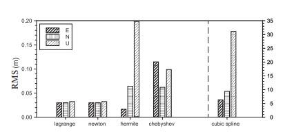
The calculation result is shown in Figure 1.
Figure 1 RMS values of different interpolation methods in ENU direction |
Full size|PPT slide
In Figure 1, RMS value of cubic spline interpolation method in E, N, U direction are 6.3210, 9.3769, 31.202, so the accuracy is poor and cannot meet the requirements. Hermite interpolation method RMS value is not large, but when the order is very high, E, N, U direction deviation will become big and have poor accuracy. RMS value of the Chebyshev fitting method are 0.1147, 0.0620, 0.0988 in respectively, its accuracy is better than Hermite interpolation method. In E, N, U direction, the accuracy are consistent between Newton interpolation method and Lagrange interpolation method and are worse than the latter three methods in this table, 0.0298, 0.0300, 0.0324.
3.3 Computation Time Length
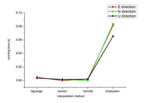
In the five interpolation methods, we can select the order which can ensure satellite position precision reach the centimeter level and obtain the operation time in respectively. The results are shown in Figure 2.
Figure 2 Computation time of different interpolation methods in ENU direction |
Full size|PPT slide
In Figure 2, Newton interpolation runs faster than the first method. Hermite interpolation method runs slightly faster than the Newton interpolation in N direction, but correspondingly, 6.3210 m, 9.3769 m, 31.202 m, especially when the interpolation times between 21 and 27, E, N, U direction deviation are big and cannot meet the requirements. The Chebyshev fitting has a slightly speed. Cubic spline interpolation method cannot reach the centimeter precision, so the computing time is not considered.
4 Conclusions
During 0:00:00–6:30:00 time, the experimental results show that E, N, U direction precision reaches centimeter when the epoch number of Newton interpolation and Lagrange interpolation is more than seven. Hermite interpolation method whose times are less than eleven can reach the accuracy of eight orders Lagrange interpolation method. Although cubic spline interpolation method has no Runge phenomenon, deviations in Table 4 are not up to the results in Table 1 and Table 2. Chebyshev fitting precision has gradually became higher owing to more epoch nodes, when the order is more than seven, the precision can reach seven orders Lagrange interpolation method. On the whole, the accuracy of cubic spline interpolation method is within meters, this method is the worst. Hermite interpolations, Chebyshev fitting method, their accuracy gradually become higher. In E, N, U direction, deviation results and RMS value of Newton and Lagrange interpolation method are equivalent, its accuracy is higher than the other three methods, moreover, it is because the running time of former is faster than the latter that the former replace the latter, in a comprehensive comparison, Newton interpolation is optimal method for satellite position solution.
{{custom_sec.title}}
{{custom_sec.title}}
{{custom_sec.content}}
 PDF(182 KB)

 Table 1 The deviation of satellite position in ENU direction obtained by Lagrange interpolation method
 Figure 1 RMS values of different interpolation methods in ENU direction


