A KELM-Based Ensemble Learning Approach for Exchange Rate Forecasting

Yunjie WEI; Shaolong SUN; Kin Keung LAI; Ghulam ABBAS

doi:10.21078/JSSI-2018-289-13

PDF(172 KB)

Journal of Systems Science and Information ›› 2018, Vol. 6 ›› Issue (4) : 289-301. DOI: 10.21078/JSSI-2018-289-13

A KELM-Based Ensemble Learning Approach for Exchange Rate Forecasting

Author information +

History +

Abstract

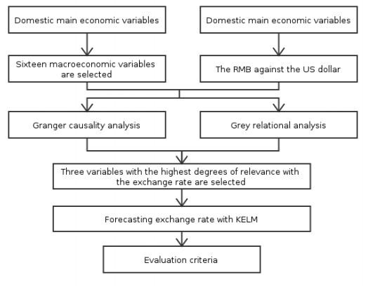
In this paper, a KELM-based ensemble learning approach, integrating Granger causality test, grey relational analysis and KELM (Kernel Extreme Learning Machine), is proposed for the exchange rate forecasting. The study uses a set of sixteen macroeconomic variables including, import, export, foreign exchange reserves, etc. Furthermore, the selected variables are ranked and then three of them, which have the highest degrees of relevance with the exchange rate, are filtered out by Granger causality test and the grey relational analysis, to represent the domestic situation. Then, based on the domestic situation, KELM is utilized for medium-term RMB/USD forecasting. The empirical results show that the proposed KELM-based ensemble learning approach outperforms all other benchmark models in different forecasting horizons, which implies that the KELM-based ensemble learning approach is a powerful learning approach for exchange rates forecasting.

Key words

exchange rate / macroeconomic variables / forecasting / kernel extreme learning machine

Cite this article

EndNote

Ris (Procite)

Bibtex

Download Citations

Yunjie WEI , Shaolong SUN , Kin Keung LAI , Ghulam ABBAS. A KELM-Based Ensemble Learning Approach for Exchange Rate Forecasting. Journal of Systems Science and Information, 2018, 6(4): 289-301 https://doi.org/10.21078/JSSI-2018-289-13

1 Introduction

Due to the deepening of the internationalization of the Renminbi(RMB), the gradual opening of the capital account and the furtherreform of the RMB pricing mechanism, the fluctuation of the RMBexchange rate has a markedly enhanced trend. With the high speed ofChina's economic development, the international influence of the RMBis increasing, and the international use of the RMB is developingrapidly. In November 2015¹, International Monetary Fund (IMF) announcedthe RMB into the Special Drawing Right (SDR) currency basket. TheRMB is now at a new stage of internationalization. According to areport of the Society for Worldwide Interbank FinancialTelecommunication (SWIFT), the RMB accounted for 2.31% of theglobal payments and was the 5th most active currency in December2015. Forecasting of exchange rate trend accurately and theanalysis of exchange rate changes scientifically are of greatsignificance in both theoretical and practical aspects.

¹Source from: https://www.swift.com

The fluctuations of the exchange rate and its impact on the economicdevelopment is an important issue in international trade andmacroeconomics. The fluctuations of the RMB exchange rates will havea significant impact on the other macroeconomic variables, andconsequently the changes in macroeconomic variables will also affectthe RMB exchange rates. According to the exchange rate pass-throughtheory, when the exchange rate pass-through is complete, themovements of nominal exchange rate will lead the price of importedgoods changes in the same proportion. The definition of exchangerate pass-through is the degree to which exchange rate changes arepassed through to price level changes between the exporting andimporting country^[1-5]. In addition, the devaluation of thecurrency will cause the government to implement the expansionarymonetary policy, which will have great impacts on the economicactivities and stock prices.

Meanwhile, the changes of macroeconomic variables will also have asignificant impact on the movements of the exchange rates. A lot ofliterature analyzed the relationship between macroeconomic variablesand the movements of exchange rates, and the selected macroeconomicvariables includs stock prices^[6-8], inflation^[9-12], import and export^[13-15], foreign exchangereserves^[16-18], etc.

The devaluation of the domestic currency will increase the price ofimported goods, thereby increasing the level of domestic inflationand so on. The fluctuations in the exchange rates will have asignificant impact on the prices of exported goods, money supply(M2), prices of imported goods, CPI, stock prices, import priceindices, PPI, etc. For different countries, the relationshipbetween the exchange rates and the macroeconomic variables aredifferent. For example, in the case of stock prices, Granger, etal.^[7] analyzed the relationship between exchange rates andstock prices in Hong Kong, Indonesia, Japan, Korea, Malaysia, Philippines, Singapore, Thailand and Taiwan during the Asian Flu.The results indicated that, 1) in Korea, the exchange rate led thestock prices; 2) the stock prices led the exchange rates to someextent in Hong Kong, Malaysia, Singapore, Thailand and Taiwan; 3)there existed no relation between the stock prices and the exchangerate market in Japan and Indonesia.

According to the existing literature, they mainly focused onanalyzing the relationship of the exchange rate with one or severalmacroeconomic variables, or comparing the differences ofinter-relationships between exchange rates and macroeconomicvariable for different countries. There are quite few studies onfiltering out the key macroeconomic variables, which have thehighest degrees of relevance with the exchange rate, to representthe domestic economic situation and to forecast the medium-termexchange rate.

In terms of historical statistics, the exchange rates show thecharacteristics of nonlinearity, uncertainty and irregularity, which make exchange rate forecasting a very challenging task.Numerous literature has been devoted to establish reliable andpromising forecasting methods to improve the forecasting ability ofexchange rate. Those methods can be divided into three categories: 1) econometric and statistical methods, including autoregressiveintegrated moving average (ARIMA) models^[19], error correctionmodels (ECM)^[20], cointegration models^[21], vectorautoregressive (VAR)^[22], generalized autoregressiveconditional heteroscedasticity (GARCH) family models^[23], etc.While the econometric and statistical methods have difficulties incapturing the nonlinear hidden patterns in the exchange rate and thecomplex interconnected relationship between the exchange rate andsome other economic factors; 2) artificial intelligent (AI) methodsincluding artificial neural network (ANN) models^[24-26], support vector regression (SVR)^[27], and deep learningtechniques^[28] are also widely employed to forecast exchangerate to avoid the limitations of these econometric and statisticalmethods; 3) by integrating a set of models, the hybrid approach canovercome the shortcomings of single models and combine the merits ofeach model to achieve a better capability^[29-31].

In this paper, a new conceptual framework with Granger causalitytest, grey relational analysis and KELM is proposed for exchangerate forecasting. Firstly, based on the existing literature, sixteenmacroeconomic variables are selected, including: Import, export, foreign exchange reserves, etc., which are often selected to studythe relationship between the exchange rate and the macroeconomicvariables. Secondly, the Granger causality test and the greyrelational analysis are employed to analyze and rank the correlationof RMB/USD with China's sixteen major macroeconomic variables. Basedon these approaches, the three variables, which have the highestdegrees of relevance with the exchange rate is further filtered outto represent the domestic economic situation. Thirdly, based on thedomestic economic situation, KELM is used to forecast the centralparity of RMB/USD.

The rest of this paper is organized as follows: Relatedmethodologies and the proposed approach are briefly introduced inSection 2. Section 3 represents the empirical results and Section 4concludes this paper.

2 Methodology

Before presenting our new approach, we introduce some methods which will be utilized in the approach.

2.1 Granger Causality Test

Granger^[32] proposed the Granger causality test, based on theassumption that there is a linear relationship between twovariables. A time series

X

is said to granger-cause another timeseries

Y

if the predication error of current

Y

declines by usingpast values of

X

in addition to past values of

Y

Let

y

and

x

be stationary time series. To test the nullhypothesis that

x

does no Granger-cause

y

, one finds the properlagged values of

y

to include in a univariate autoregression of

y

\begin{array}{rcl} y_{t} & = & α_{0} + α_{1} y_{t - 1} + \dots + α_{m} y_{t - m} + ε_{t} . \end{array}

(1)

Next, the autoregression is augmented by including lagged values of

x

\begin{array}{rcl} y_{t} & = & α_{0} + α_{1} y_{t - 1} + \dots + α_{m} y_{t - m} + β_{p} x_{t - p} + \dots + β_{q} x_{t - q} + ε_{t} . \end{array}

(2)

One retains in this regression all lagged values of

x

that areindividually significant according to their

t

-statistics, provided that collectively they add explanatory power to theregression according to an

F

-test (whose null hypothesis is noexplanatory power jointly added by the

x^{'} s

). In the notation ofthe above augmented regression,

p

is the shortest, and

q

is thelongest, lag length for which the lagged value of

x

issignificant.

The null hypothesis that

x

does not Granger-cause

y

is acceptedif and only if no lagged values of

x

are retained in theregression. The Granger causality test has been widely used toanalyze the relationship of economic and financial variables. Forfurther details on this method, please refer to Granger^[32].

2.2 Grey Relational Analysis

Grey relational analysis is employed to solve problems withcomplicated interrelationships between multiple variables, which isa measurement method to determine the relationship between sequencesusing limited amounts of data.

The grey relational coefficient and grey relational degree can be formulated as follows:

\begin{array}{rcl} γ_{0 i} (k) = \frac{m + ξ max_{i} max_{k} | x_{0}^{'} (k) - x_{i}^{'} (k) |}{| x_{0}^{'} (k) - x_{i}^{'} (k) | + ξ max_{i} max_{k} | x_{0}^{'} (k) - x_{i}^{'} (k) |}, \end{array}

(3)

\begin{array}{rcl} γ_{0 i} = \frac{1}{n} \sum_{k = 1}^{n} γ_{0 i} (k), \end{array}

(4)

where

ξ \in (0, 1); k = 1, 2, \dots, n; i = 1, 2, \dots, m .

The fundamentalidea of the grey relational analysis is that the closeness of arelationship is judged based on the similarity level of thegeometric patterns of sequence curves. Then the variables are rankedby the degree of relevance. The higher the degree of geometricsimilarity, the greater the degree of correlation^{[33, 34]}.

2.3 Kernel Extreme Learning Machine (KELM)

Huang^[35] further extended the Extreme Learning Machine (ELM)and proposed Kernel Extreme Learning Machine (KELM). ELM is thesingle layer feed-forward neural network (SLFN) architecture. Themain drawbacks of ELM are that it has the random initialization andits prediction precision is very sensitive to the noise and thenumber of hidden layer nodes, which will lead to a poor robustness.Therefore, KELM is proposed to overcome the disadvantages of basicELM with faster convergence speed, multi-output, better stabilityand generalization ability. KELM is widely used in global solarradiation prediction, illumination correction, wind forecasting, etc^[36-38]. However, KELM has not been used yet in the exchangerate forecasting. For given

N

sample

(x_{i}, y_{i})

with

L

hiddenneurons,

x_{i} \in R^{N}

is the input vector,

y_{i} \in R^{N}

is thecorresponding output vector, and

h (x)

is the activationfunction, the output function of ELM can be defined as:

\begin{array}{rcl} f (x) = \sum_{i = 1}^{L} β_{i} h_{i} (x) = h (x) β, \end{array}

(5)

where,

H = h_{i j}

is the hidden layer output matrixof neural network,

β = [β_{1}, β_{2}, \dots, β_{L}]

is theoutput weight connecting hidden nodes to output nodes.

The output weights can be calculated by the least square method:

\begin{array}{rcl} β = H^{+} T, \end{array}

(6)

where,

H^{+}

is the Moore-Penrose generalized inverseof matrix

H

(Huang, et al.^[39]).

According to the Karush-Kuhn-Tucker (KKT) theorem, it can be writtenas

\begin{array}{rcl} β = H (\frac{I}{C} + H H^{\rmT})^{- 1} T . \end{array}

(7)

The output function can be formulated as follows:

\begin{array}{rcl} f (x) = h (x) H (\frac{I}{C} + H H^{\rmT})^{- 1} T . \end{array}

(8)

Huang, et al.^[39] introduced the kernel function in ELM and byapplying Mercer's conditions on ELM, a kernel matrix for ELM can beformulated as follows:

\begin{array}{rcl} Ω_{E L M} = H H^{T} : Ω_{\rmELM_{i, j}} = h (x_{i}) h (x_{j}) = K (x_{i}, x_{j}), \end{array}

(9)

where

i, j = 1, 2, \dots, N

;

K (x_{i}, x_{j})

is a kernel function.The output function of KELM can be formulated as follows:

\begin{array}{rcl} f (x) = h (x) H (\frac{I}{C} + H H^{\rmT})^{- 1} T = {[\begin{array}{c} K (x, x_{1}) \\ ⋮ \\ K (x, x_{N}) \end{array}]}^{T} (\frac{I}{C} + Ω_{E L M})^{- 1} T . \end{array}

(10)

From the above equations, it can be derived that by introducing thekernel function into ELM to get the least-squares optimal solution, which leads to a better generalization performance and more stablethan basic ELM. For further details on this method, please refer toHuang^[35].

2.4 KELM-Based Ensemble Learning Approach

In this paper, a KELM-based ensemble learning approach integratingGranger causality test, grey relational analysis and KELM isproposed for exchange rate forecasting, as shown in Figure 1. Thisframework mainly describes a modeling process that starts from dataextraction, data fusion and data computing. The proposed KELM-basedensemble learning approach includes the following three steps:

Figure 1 A KELM-based ensemble learning approach.

Full size|PPT slide

Step 1 Data extraction. According to the existingliterature, sixteen macroeconomic variables are selected, including:import, export, foreign exchange reserves, etc., which are often selected to study the relationship between the exchange rate and the macroeconomic variables.

Step 2 Data fusion. By integrating Granger causalitytest and Grey relational analysis, we rank the correlation ofRMB/USD with the China's sixteen major macroeconomic variables, andthen filter the three variables which have the highest degrees ofrelevance with the exchange rate to represent the domesticsituation.

Step 3 Data computing. Based on the domestic situation, KELM is used to forecast the central parity of RMB/USD. And multipleevaluation criteria are employed to comprehensively evaluate theforecasting performance of the proposed approach and benchmarks.

3 Empirical Study

3.1 Data Collection

According to the existing literature, sixteen macroeconomic variables, which have higher degreesof relevance with the RMB against US dollar (RMB/USD), are selected, including: Import (IM), export (EX), import growth (IM_YOY), export growth (EX_YOY), import price index (IPI), export price index (EPI), foreign exchange reserves (FER), growth of foreign exchange reserves (FER_YOY), consumer price index (CPI), producer price index (PPI), retail price index (RPI), money supply (M2), growth of money supply (M2_YOY), industrial value added (IVA), Shenzhen composite index (SZCOMP) and the Shanghai composite index (SHCOMP).

The RMB exchange rate regime has been reformed several times. In July 2008, in order to preserve exchange rate stability in China and helped China's economy ride through the impact of the US subprime mortgage crisis, the China's central bank pegged the RMB against the US dollar at 6.83 and narrowed the floating range of the RMB exchange rate. In June 19, 2010, China's central bank announced to resume and further the reform of the RMB exchange rate regime based on measures taken in 2005, to increase the flexibility of the RMB exchange rate. Since the RMB against the US dollar was pegged at 6.83 from the middle of 2008 to June 2010, the monthly data used in this paper are obtained from the Wind Database (http://www.wind.com.cn/), covering the period from July 2010 to July 2017. The data are divided into in-sample subset and out-of-sample subset: 1) The in-sample subset is used for model training with data from July 2010 to January 2017; 2) The out-of-sample subset is used for empirical testing with data ranging from February 2017 to July 2017. The detailed data are not listed here but can be obtained from the Wind Database or from the authors.

A logarithmic transformation is applied to IM, EX, FER, M2, SZCOMPand SHCOMP, named IM_LN, EX_LN, FER_LN, M2_LN, SZ_LN and SH_LN. The descriptive statistics of the selected variables are displayed in Table 1. It clearly indicates the difference in the statistical features among the subsets. Skewness analysis is utilized to depict the symmetry of the subset. For skewness, the greater the absolute skewness value is, the more obvious the asymmetry is. And kurtosis is used to depict the steepness of the subset. For kurtosis, values greater than 0 indicate that the distribution of the dataset is steeper than the standard Gaussian distribution.

Table 1 Statistical properties of the domestic economic variables and the exchange rate

Variable	Mean	Standard Deviation	Skewness	Kurtosis	Jarque-Bera	P value	Observations
RMB/USD	6.40	0.25	0.60	2.15	7.75	0.02	85
IM_LN	7.28	0.13	-0.82	3.91	12.45	0.00	85
EX_LN	7.46	0.16	-1.28	5.09	38.87	0.00	85
IM_YOY	6.26	16.18	0.39	2.65	2.55	0.28	85
EX_YOY	7.46	13.77	0.43	3.40	3.20	0.20	85
IPI	100.77	8.94	0.21	1.98	4.32	0.12	85
EPI	101.87	4.46	0.63	2.43	6.71	0.03	85
FER_LN	10.42	0.11	-0.21	2.76	0.84	0.66	85
FER_YOY	4.43	12.41	0.18	2.02	3.83	0.15	85
CPI	2.68	1.41	1.14	3.37	18.88	0.00	85
PPI	0.05	4.31	0.53	1.88	8.33	0.02	85
RPI	1.77	1.68	1.11	3.17	17.44	0.00	85
M2_LN	13.91	0.26	-0.21	1.86	5.23	0.07	85
M2_YOY	13.54	2.25	0.76	3.83	10.65	0.00	85
IVA	9.13	3.49	0.68	3.62	7.95	0.02	85
SZ_LN	7.19	0.33	0.39	1.81	7.16	0.03	85
SH_LN	7.89	0.20	0.51	2.71	3.96	0.14	85

3.2 Correlation Analysis

In this section, we estimate the degrees of relevance by using the monthly datasetsof those sixteen macroeconomic variables and the central parity of RMB/USD by granger causality test and grey relational analysis.

3.2.1 Granger Causality Test

Since the test is sensitive to the lag order, the Akaike informationcriterion (AIC) and Schwarz information criterion (SC) are used inthis section to determine the optimal lag order.

Table 2 shows the results of the Granger causality test of thecentral parity of RMB/USD and the major domestic economic variables, which indicates that under 5% significant level, EX_LN, PPI, RPI, FER_LN, SZ_LN and SH_LN granger cause RMB/USD, vice versa. The movements of RMB/USD will cause the fluctuations of EX_LN, PPI, RPI, FER_LN, SZ_LN and SH_LN, and the changes in EX_LN, PPI, RPI, FER_LN, SZ_LN and SH_LN will also have impact on RMB/USD.

Table 2 Results of the Granger causality test

	F-Statistic	Prob.
IM_LN does not Granger Cause RMB/USD	0.090	0.765
RMB/USD does not Granger Cause IM_LN	8.935	0.004^***
EX_LN does not Granger Cause RMB/USD	5.416	0.023^**
RMB/USD does not Granger Cause EX_LN	4.389	0.040^**
IM_YOY does not Granger Cause RMB/USD	2.637	0.079
RMB/USD does not Granger Cause IM_YOY	5.009	0.009^***
EX_YOY does not Granger Cause RMB/USD	14.491	0.000^***
RMB/USD does not Granger Cause EX_YOY	1.154	0.286
IPI does not Granger Cause RMB/USD	1.140	0.349
RMB/USD does not Granger Cause IPI	4.256	0.002^***
EPI does not Granger Cause RMB/USD	1.096	0.371
RMB/USD does not Granger Cause EPI	4.272	0.002^***
FER_LN does not Granger Cause RMB/USD	5.976	0.017^***
RMB/USD does not Granger Cause FER_LN	9.761	0.003^***
FER_YOY does not Granger Cause RMB/USD	2.121	0.074
RMB/USD does not Granger Cause FER_YOY	1.855	0.115
CPI does not Granger Cause RMB/USD	2.888	0.062
RMB/USD does not Granger Cause CPI	6.684	0.002^***
PPI does not Granger Cause RMB/USD	4.175	0.009^***
RMB/USD does not Granger Cause PPI	5.122	0.003^***
RPI does not Granger Cause RMB/USD	3.566	0.018^***
RMB/USD does not Granger Cause RPI	4.044	0.010^***
M2_LN does not Granger Cause RMB/USD	6.436	0.003^***
RMB/USD does not Granger Cause M2_LN	0.064	0.939
M2_YOY does not Granger Cause RMB/USD	2.282	0.057
RMB/USD does not Granger Cause M2_YOY	0.507	0.770
IVA does not Granger Cause RMB/USD	4.531	0.006^***
RMB/USD does not Granger Cause IVA	1.874	0.142
SZ_LN does not Granger Cause RMB/USD	7.051	0.000^***
RMB/USD does not Granger Cause SZ_LN	3.678	0.016^**
SH_LN does not Granger Cause RMB/USD	3.442	0.021^**
RMB/USD does not Granger Cause SH_LN	2.750	0.049^**

Notes: ^*** represent under 1% significant level
^** represent under 5% significant level

A considerable amount of literature shows that with the opening ofthe capital market, the appreciation of domestic currency would leadthe stock prices to rise. Otherwise, the foreign exchange market will affect the stock market mainly through four channels: 1) Foreign exchange rate may affect the stock prices through the liquidity of stock market; 2) Exchange rate fluctuations will affect the adjustment of the government's economic policy, through policy-oriented changes, and the exchange rate can affect the stock prices; 3) The exchange rate may also influence the substitution of investors' portfolios, which will lead to the change of supply and demand relationships of different assets, and stock prices will be affected; (4) export-oriented enterprises have many account receivable and assets of foreign currency accounts. If domestic currency is devalued, those assets and account receivable will be appreciated. On the contrary, the export-oriented enterprises also have many foreign currency liabilities. If domestic currency is devalued, foreign currency liabilities will increase, which will have a negative impact on the stock prices of those enterprises. It has been confirmed by many studies on the Granger causality of RMB/USD and PPI, export growth and stock price^{[7, 8]}.

While, RMB/USD granger cause IM_LN, IM_YOY, IPI, EPI and CPI, which means the movements of RMB/USD will have impact on the logimport, growth of import, import price index, export price index, consumer price index. And EX_YOY, M2_LN, IVA also granger causeRMB/USD.

3.2.2 Grey Relational Analysis

Table 3 shows the results of the grey relational analysis. The four variables with the highest degrees of relevance with RMB/USD are SZ_LN, FER_LN, IM_LN and EX_LN, with the relevant degrees of 0.813, 0.800, 0.775 and 0.726, respectively. Both variables, i.e., EX_LN and IM_LN belong to foreign trade, and the gray relevant degrees of them are similar. However, EX_LN granger cause RMB/USD, and vice versa. Therefore, EX_LN is selected in the model.

Table 3 Results of the grey relational analysis of RMB/USD and domestic economic variables

Variables	Correlation Degree	Variables	Correlation Degree
IM_LN	0.775	CPI	0.711
EX_LN	0.726	PPI	0.535
IM_YOY	0.528	RPI	0.657
EX_YOY	0.524	M2_LN	0.771
IPI	0.648	M2_YOY	0.604
EPI	0.653	IVA	0.580
FER_LN	0.800	SZ_LN	0.813
FER_YOY	0.533	SH_LN	0.5815

Based on these approaches, FER_LN, SZ_LN and EX_LN are selected to represent the majordomestic macroeconomic variables and to forecast the central parity of the RMB against the US dollar.

3.3 Evaluation Criteria

In order to effectively evaluate the forecasting performance of the proposed KELM-basedensemble learning approach, four models are utilized as benchmarks, including the autoregressive moving average model (ARIMA), random walk (RW), autoregressive model (VAR) and least squares support vector regression (LSSVR).

Meanwhile, the mean absolute percentage error (MAPE) and the root mean square error (RMSE) are employed to evaluate the level of forecasting accuracy. The specific formulas are as follows^[31]:

\begin{array}{rcl} M A P E = \frac{1}{n} \sum_{t = 1}^{n} | \frac{Y_{t} - \hat{Y_{t}}}{Y_{t}} | \times 100 %, \end{array}

(11)

\begin{array}{rcl} \rmRMSE = \sqrt{\frac{1}{n} \sum_{t = 1}^{n} (Y_{t} - \hat{Y_{t}})^{2}}, \end{array}

(12)

where

Y_{t}

and

\hat{Y_{t}}

represent the actual value andthe forecast value at time

t

respectively, and

n

is the numberof observations. The MAPE and RMSE are utilized to measure thedeviation between the actual value and the forecasting value and thesmaller values represent the higher accuracy^[31].

3.4 KELM-Based Ensemble Learning Approach

3.4.1 Performance Comparison

To this section, the KELM-based ensemble learning approach with thethree selected variables (FER_LN, SZ_LN and EX_LN), is proposedto forecast the monthly central parity of the RMB against the USdollar. These three variables, i.e., FER_LN, SZ_LN and EX_LN arerepresenting the domestic economic situation. Meanwhile theforecasting performances of the proposed approach and benchmarks arediscussed.

The forecasting performance comparison of MAPE, RMSE and DSevaluation criteria are listed in Tables 4–6. From theseresults, it can be easily concluded that the forecasting performanceof KELM-based ensemble learning approach can significantlyoutperform all of the benchmark models, which obtains the smallestMAPE and RMSE in different frequencies for exchange rateforecasting.

Table 4 One-month-ahead forecasting results on monthly RMB/USD

Models	RW	ARIMA	VAR	LSSVR	KELM
MAPE (%)	0.1920	0.3212	0.3277	0.2232	0.1515
RMSE	0.1319	0.2207	0.2252	0.1534	0.1041

Table 5 Three-month-ahead forecasting results on monthly RMB/USD

Models	RW	ARIMA	VAR	LSSVR	KELM
MAPE (%)	0.4122	0.1736	0.2019	0.5301	0.1691
RMSE	0.3198	0.1454	0.1610	0.4038	0.1397

Table 6 Six-month-ahead forecasting results on monthly RMB/USD

Models	RW	ARIMA	VAR	LSSVR	KELM
MAPE (%)	0.6574	0.6981	0.5917	0.5620	0.2236
RMSE	0.5686	0.6937	0.5508	0.4105	0.2098

The performance of machine learning approaches, such as KELM andLSSVR, are better than the econometric and statistical models.Since the exchange rate data show the characteristics ofnonlinearity, uncertainly and irregularity, so the machine learningtechniques are much more appropriate than ARIMA, VAR and RM forexchange rate forecasting.

In specific, three main conclusions can be summarized: 1) Theproposed KELM-based ensemble learning approach outperforms all otherbenchmark models in different forecasting horizons, which impliesthat the KELM-based ensemble learning approach is a powerfullearning approach for exchange rates forecasting; 2) Theforecasting performance of the proposed ensemble learning approachis significantly better than single model. The possible reason isthat the approach can utilize more information of the domesticeconomic situation, which will help to dramatically improve theforecasting performance of single models; 3) Due to thenonlinearity, irregularity of the exchange rate data, theperformance of machine learning approaches, such as KELM and LSSVR, are better than the econometric and statistical models.

4 Conclusions

In this paper, a KELM-based ensemble learning approach, integratingGranger causality test, grey relational analysis and KELM, isproposed for exchange rate forecasting. The framework of theproposed approach includes three steps. First, the data extraction, according to the existing literature, a set of sixteen macroeconomicvariables is selected, including: Import, export, foreign exchangereserves, etc. Second, data fusion, we rank the selected sixteenmacroeconomic variables and filter out three of them, which have thehighest degrees of relevance with the exchange rate to represent thedomestic situation by using Granger causality test and the greyrelational analysis. Third, data computing, based on the domesticsituation, KELM is utilized for medium-term RMB/USD forecasting. Theempirical results show that the proposed KELM-based ensemblelearning approach outperforms all other benchmark models indifferent forecasting horizons which implies that the KELM-basedensemble learning approach is a powerful learning approach forexchange rates forecasting.

References

Publishing order | Descend order by publishing year | Descend order by cited within

1	Goldberg P K, Knetter M M. Goods prices and exchange rates: What have we learned?. Journal of Economic Literature, 1997, 35, 1243- 1272. Cited in this article [1]

2	Campa J M, Goldberg L S. Exchange rate pass-through into import prices: A macro or micro phenomenon?. National Bureau of Economic Research, 2002.

3	Campa J M, Goldberg L S. Exchange-rate pass-through into import prices. Review of Economics and Statistics, 2005, 87 (4): 679- 690. https://doi.org/10.1162/003465305775098189

4	Jiang J, Kim D. Exchange rate pass-through to inflation in China. Economic Modelling, 2013, 33, 900- 912. https://doi.org/10.1016/j.econmod.2013.05.021

5	Abbas G, Bhowmik R, Koju L, et al. Cointegration and causality relationship between stock market, money market and foreign exchange market in Pakistan. Journal of Systems Science and Information, 2017, 5 (1): 1- 20. https://doi.org/10.21078/JSSI-2017-001-20 Cited in this article [1]

6	Abdalla I S A, Murinde V. Exchange rate and stock price interactions in emerging financial markets: Evidence on India, Korea, Pakistan and the Philippines. Applied Financial Economics, 1997, 7 (1): 25- 35. https://doi.org/10.1080/096031097333826 Cited in this article [1]

7	Granger C W J, Huangb B N, Yang C W. A bivariate causality between stock prices and exchange rates: Evidence from recent Asian flu. The Quarterly Review of Economics and Finance, 2000, 40 (3): 337- 354. https://doi.org/10.1016/S1062-9769(00)00042-9 Cited in this article [2]

8	Aydemir O, Demirhan B. The relationship between stock prices and exchange rates: Evidence from MENA countries. Handbook of Research on Global Enterprise Operations and Opportunities. IGI Global, 2017, 171- 185. Cited in this article [2]

9	Mccarthy J. Pass-through of exchange rates and import prices to domestic inflation in some industrialized economies. Staff Reports No. 111, Federal Reserve Bank of New York, 2000. Cited in this article [1]

10	Ito T, Sato K. Exchange rate changes and inflation in post-crisis Asian economies: Vector autoregression analysis of the exchange rate pass-through. Journal of Money, Credit and Banking, 2008, 40 (7): 1407- 1438. https://doi.org/10.1111/j.1538-4616.2008.00165.x

11	Lin S, Ye H. Does inflation targeting make a difference in developing countries?. Journal of Development Economics, 2009, 89 (1): 118- 123. https://doi.org/10.1016/j.jdeveco.2008.04.006

12	Romero F P. How does the Philippine peso exchange rate respond to inflation, industrial production and trade balance? A Granger causality analysis. Advanced Science Letters, 2017, 23 (1): 272- 276. https://doi.org/10.1166/asl.2017.7155 Cited in this article [1]

13	Bini-Smaghi L. Exchange rate variability and trade: Why is it so difficult to find any empirical relationship?. Applied Economics, 1991, 23 (5): 927- 936. https://doi.org/10.1080/00036849100000041 Cited in this article [1]

14	Chowdhury A R. Does exchange rate volatility depress trade flows? Evidence from error-correction models. The Review of Economics and Statistics, 1993, 700- 706.

15	Doganlar M. Estimating the impact of exchange rate volatility on exports: Evidence from Asian countries. Applied Economics Letters, 2002, 9 (13): 859- 863. https://doi.org/10.1080/13504850210150906 Cited in this article [1]

16	Eichengreen M B J, Mathieson M D J. The currency composition of foreign exchange reserves: Retrospect and prospect. International Monetary Fund, 2000. Cited in this article [1]

17	Jiang J, Kim D. Exchange rate pass-through to inflation in China. Economic Modelling, 2013, 33, 900- 912. https://doi.org/10.1016/j.econmod.2013.05.021

18	Bhattacharya R, Patnaik H, Shah A. Monetary policy transmission in an emerging market setting. IMF Working Paper No. 11/5, International Monetary Fund, Washington D.C., 2011. Cited in this article [1]

19	Chortareas G, Jiang Y, Nankervis J C. Forecasting exchange rate volatility using high-frequency data: Is the euro different?. International Journal of Forecasting, 2011, 27 (4): 1089- 1107. https://doi.org/10.1016/j.ijforecast.2010.07.003 Cited in this article [1]

20	Moosa I A, Vaz J J. Cointegration, error correction and exchange rate forecasting. Journal of International Financial Markets, Institutions and Money, 2016, 44, 21- 34. https://doi.org/10.1016/j.intfin.2016.04.007 Cited in this article [1]

21	McCrae M, Lin Y X, Pavlik D, et al. Can cointegration-based forecasting outperform univariate models? An application to Asian exchange rates. Journal of Forecasting, 2002, 21 (5): 355- 380. https://doi.org/10.1002/for.824 Cited in this article [1]

22	Joseph N L. Model specification and forecasting foreign exchange rates with vector autoregressions. Journal of Forecasting, 2001, 20 (7): 451- 484. https://doi.org/10.1002/for.808 Cited in this article [1]

23	Roni B, Wu C, Jewel R K, et al. A Study on the volatility of the Bangladesh stock marketbased on GARCH type models. Journal of Systems Science and Information, 2017, 5 (3): 193- 215. https://doi.org/10.21078/JSSI-2017-193-23 Cited in this article [1]

24	Hu M Y, Zhang G P, Jiang C X, et al. A Cross-Validation analysis of neural network out-of-sample performance in exchange rate forecasting. Decision Sciences, 1999, 30 (1): 197- 216. https://doi.org/10.1111/j.1540-5915.1999.tb01606.x Cited in this article [1]

25	Raji C G, Chandra S S V. Long-term forecasting the survival in liver transplantation using multilayer perceptron networks. IEEE Transactions on Systems, Man, and Cybernetics: Systems, 2017, 47 (8): 2318- 2329. https://doi.org/10.1109/TSMC.2017.2661996

26	Li X, Zhang Z, Huang C. An EPC forecasting method for stock index based on integrating empirical mode decomposition, SVM and Cuckoo search algorithm. Journal of Systems Science and Information, 2014, 2 (6): 481- 504. https://doi.org/10.1515/JSSI-2014-0481 Cited in this article [1]

Sermpinis G, Stasinakis C, Theofilatos K, et al. Modeling, forecasting and trading the EUR exchange rates with hybrid rolling genetic algorithms-Support vector regression forecast combinations. European Journal of Operational Research, 2015, 247 (3): 831- 846.

https://doi.org/10.1016/j.ejor.2015.06.052

Cited in this article [1]

28	Shen F, Chao J, Zhao J. Forecasting exchange rate using deep belief networks and conjugate gradient method. Neurocomputing, 2015, 167, 243- 253. https://doi.org/10.1016/j.neucom.2015.04.071 Cited in this article [1]

Yu L, Lai K K, Wang S. Multistage RBF neural network ensemble learning for exchange rates forecasting. Neurocomputing, 2008, 71 (16): 3295- 3302.

http://www.researchgate.net/profile/Lean_Yu/publication/222054065_Multistage_RBF_neural_network_ensemble_learning_for_exchange_rates_forecasting/links/0f3175332e4da45c4d000000.pdf

Cited in this article [1]

30	Yu L, Wang S, Lai K K. Forecasting crude oil price with an EMD-based neural network ensemble learning paradigm. Energy Economics, 2008, 30 (5): 2623- 2635. https://doi.org/10.1016/j.eneco.2008.05.003

31	Sun S L, Qiao H, Wei Y J, et al. A new dynamic integrated approach for wind speed forecasting in China. Applied Energy, 2017, 197, 151- 162. https://doi.org/10.1016/j.apenergy.2017.04.008 Cited in this article [3]

32	Granger C. Investigating causal relations by econometric models and cross-spectral methods. Econometrica, 1969, 37 (3): 424- 438. https://doi.org/10.2307/1912791 Cited in this article [2]

33	Tan X, Yang Y, Deng J. Grey relational analysis factors in hypertensive with cardiac insufficiency. Journal of Grey System, 1998, 10 (1): 75- 80. Cited in this article [1]

34	Kao P S, Hocheng H. Optimization of electrochemical polishing of stainless steel by grey relational analysis. Journal of Materials Processing Technology, 2003, 140 (1): 255- 259. Cited in this article [1]

35	Huang G B. An insight into extreme learning machines: Random neurons, random features and kernels. Cognitive Computation, 2014, 6 (3): 376- 390. https://doi.org/10.1007/s12559-014-9255-2 Cited in this article [2]

36	Zhou Z, Xu R, Wu D, et al. Illumination correction of dyeing products based on Grey-Edge and kernel extreme learning machine. Optik-International Journal for Light and Electron Optics, 2016, 127 (19): 7978- 7985. https://doi.org/10.1016/j.ijleo.2016.05.108 Cited in this article [1]

37	Shamshirband S, Mohammadi K, Chen H L, et al. Daily global solar radiation prediction from air temperatures using kernel extreme learning machine: A case study for Iran. Journal of Atmospheric and Solar-Terrestrial Physics, 2015, 134, 109- 117. https://doi.org/10.1016/j.jastp.2015.09.014

38	Sun S L, Wang S Y, Wei Y J, et al. A clustering-based nonlinear ensemble approach for exchange rates forecasting. IEEE Transactions on Systems, Man, and Cybernetics: Systems, 2018. https://doi.org/10.1109/TSMC.2018.2799869 Cited in this article [1]

39	Huang G B, Zhu Q Y, Siew C K. Extreme learning machine: Theory and applications. Neurocomputing, 2006, 70 (1-3): 489- 501. https://doi.org/10.1016/j.neucom.2005.12.126 Cited in this article [2]

Funding

the National Natural Science Foundation of China(71373262)

PDF(172 KB)

198

Accesses

Citation

Detail

Sections

Recommended

Abstract
Key words
Cite this article
1 Introduction
2 Methodology
2.1 Granger Causality Test
2.2 Grey Relational Analysis
2.3 Kernel Extreme Learning Machine (KELM)
2.4 KELM-Based Ensemble Learning Approach
Figure 1 A KELM-based ensemble learning approach.
3 Empirical Study
3.1 Data Collection
Table 1 Statistical properties of the domestic economic variables and the exchange rate
3.2 Correlation Analysis
3.2.1 Granger Causality Test
Table 2 Results of the Granger causality test
3.2.2 Grey Relational Analysis
Table 3 Results of the grey relational analysis of RMB/USD and domestic economic variables
3.3 Evaluation Criteria
3.4 KELM-Based Ensemble Learning Approach
3.4.1 Performance Comparison
Table 4 One-month-ahead forecasting results on monthly RMB/USD
Table 5 Three-month-ahead forecasting results on monthly RMB/USD
Table 6 Six-month-ahead forecasting results on monthly RMB/USD
4 Conclusions
References
Funding

Received	Accepted	Published
2018-01-05	2018-03-10	2018-08-25
Issue Date
2018-08-25

Please choose a citation manager

Content to export

Abstract

Key words

Cite this article

1 Introduction

2 Methodology

2.1 Granger Causality Test

2.2 Grey Relational Analysis

2.3 Kernel Extreme Learning Machine (KELM)

2.4 KELM-Based Ensemble Learning Approach

Figure 1 A KELM-based ensemble learning approach.

3 Empirical Study

3.1 Data Collection

Table 1 Statistical properties of the domestic economic variables and the exchange rate

3.2 Correlation Analysis

3.2.1 Granger Causality Test

Table 2 Results of the Granger causality test

3.2.2 Grey Relational Analysis

Table 3 Results of the grey relational analysis of RMB/USD and domestic economic variables

3.3 Evaluation Criteria

3.4 KELM-Based Ensemble Learning Approach

3.4.1 Performance Comparison

Table 4 One-month-ahead forecasting results on monthly RMB/USD

Table 5 Three-month-ahead forecasting results on monthly RMB/USD

Table 6 Six-month-ahead forecasting results on monthly RMB/USD

4 Conclusions

{{custom_sec.title}}

{{custom_sec.title}}

References

{{custom_fnGroup.title_en}}

Footnotes

Funding

Share

模态框（Modal）标题

Please choose a citation manager

Content to export

Abstract

Key words

Cite this article

1 Introduction

2 Methodology

2.1 Granger Causality Test

2.2 Grey Relational Analysis

2.3 Kernel Extreme Learning Machine (KELM)

2.4 KELM-Based Ensemble Learning Approach

Figure 1 A KELM-based ensemble learning approach.

3 Empirical Study

3.1 Data Collection

Table 1 Statistical properties of the domestic economic variables and the exchange rate

3.2 Correlation Analysis

3.2.1 Granger Causality Test

Table 2 Results of the Granger causality test

3.2.2 Grey Relational Analysis

Table 3 Results of the grey relational analysis of RMB/USD and domestic economic variables

3.3 Evaluation Criteria

3.4 KELM-Based Ensemble Learning Approach

3.4.1 Performance Comparison

Table 4 One-month-ahead forecasting results on monthly RMB/USD

Table 5 Three-month-ahead forecasting results on monthly RMB/USD

Table 6 Six-month-ahead forecasting results on monthly RMB/USD

4 Conclusions

{{custom_sec.title}}

{{custom_sec.title}}

References

{{custom_fnGroup.title_en}}

Footnotes

Funding