1 Introduction
Attention has been dedicated to ''drone'', which is also named Unmanned Aerial Vehicles (UAVs, aircrafts piloted by remote control or onboard computers as in the Oxford Dictionary), It recently becomes widely available in the commercial marketplace. The quadcopter is a special kind of drone, which has four rotors. The UAV has been applied to commercial use test by Amazon, DHL, JD etc. There are articles that talk about how it works. Gatteschi, Lamberti, et al.
[1] explained how it works for quadcopter to delivery drugs. We try to give a solution to optimization of the quadrotor's route in delivering the e-commerce parcels in rural town or village. Due to the limited flying distance of drone, a truck drone in tandem system is introduced. Considering the relationship of traditional vehicle routing problem, we define our research problem as drones traveling salesman problem (DTSP).
2 Literature Review
There are literatures about using drone or quadcopter as way to delivery parcels. Hong, Kuby, et al.
[2] showed us the usage of commercial drone in the urban area. The research considers the battery recharging problem and tries to build a network to cover the urban city. It also considers the barrier problem. The model is based on the Euclidean shortest path problem, which has been solved Lee and Preparata
[3]. There are also literatures about the internal logistic usage of quadcopter. Olivares, Cordova, et al.
[4] talked about the quadcopters' usage inside a manufacturing plant. The research uses the sweep algorithm; it divides the process into two steps. In the first phase the clusters are formed. In the second phase, the problem is transformed into traveling sales man problem. There are literatures about the truck-drone in tandem delivery network. Ferrandez, Harbison, et al.
[5] has found that the truck-drone in tandem delivery network is better than truck or drones work alone. The research also gives us the best number of launch locations and the best of number of drones on the truck. In this article, we also adopt this tandem mode. We first cluster the demand dots, then we do a TSP problem, which is about depot and cluster center. Besides the new research on quadcopters' usage and optimization, the traditional research about the vehicle routing problem can also be applied to this new scenario. Some research is helpful to solve QRP problem. Ombuki, Ross, et al.
[6] has researched the multi-objective vehicle routing problem with time window. Baldacci, Toth, et al.
[7] has done an study about the vehicle routing problem with a capacity constraints. The work most closely related to DTSP appears to Murray, et al.
[8]. It brings two models: The flying sidekick TSP and the parallel drone scheduling TSP. It models a tandem system in FSTSP, the depot is far from the customer. The truck can recharge a drone. Both the truck and drone can serve customers. The truck meets the drone at customer demand location. Our work is different from that in following aspect. First, we define multiple drones problem, more than one drone is used in our work. Second, the truck stays at the centroids is not working for delivery. Third, we do not consider the case that the demand point cannot served by drone. We think the payload of drone is capable to handling most parcels. The drone fly range problem can be solved by the truck drone in tandem system.
3 Model
Assumptions is put forward. The following operating conditions are assumed:
1) The truck is staying still while the drone in the route, therefore the drones can be recharged and go to another round of delivering.
2) The drones use the truck as harbors, it can serve the drone many times and the recharging time is tiny, which can be omitted in our cases.
3) The drones arrive at the demand points in a direct line way, which means it is an Euclidean distance in calculation between the demand points and the truck.
4) The demand points are reached once and only once by drones (other than the depot, of course).
5) The demand points are far from the depot, so it is not applicable to launch the drones from the depot directly.
Objective: Find the solution that saves energy and time with shorter truck route. The flight height of drone is about 300 meters. The payload is required no more than 5 pounds; the maximum flight radius is about 20 km. Here we do not consider the flight control and mechanical problem such as moving direction etc. We use random number from the computer. We get random 150 demand dots through random function with code. The large number of demand points are served by the drone and truck in tandem system
[9, 10]. So we get the demand dot data
.
= [randn(50,2) + ones(50,2); randn(50,2)
ones(50,2); randn(50,2) + [ones(50,1),
ones(50,1)]]; The depot is far from most of the demand dots. In our case, the depot O location is set at
.
4 Drone Vehicle Routing Problem Solution
The design of the algorithm herein computes the minimal time of delivery.
-means clustering is used to find cluster centroid, which is the drone's launch locations
[11].
We design a drone vehicle problem. We can get the number of clusters by referring the total demand area and the flight capacity area of drone, as shown in Equation (4.1).
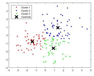
In our study case, the total number of cluster is 3. We use -means method to solve a 3 clusters problem. The clustering code is shown in the following. The clustering can be seen in Figure 1.
Figure 1 Demand point clustering |
Full size|PPT slide
Get the 150 random dot
=[randn(50,2) + ones(50,2); randn(50,2) ones(50,2); randn(50,2) + [ones(50,1), ones(50,1)] opts=statset('Display', 'final');
Apply -means function
the demand coordination
Idx vector, storage of the cluster label
Ctrs rectangle, storage of the coordination of the centroids
SumD vector, storage each cluster sum of all demand points to their centroids
D rectangle, storage all demand points to their centroids
[Idx,Ctrs,SumD,]=kmeans(,3,'Replicate',3,'Options',opts);
plot(X(Idx==1,1),X(Idx==1,2),'r.','MarkerSize',14)
hold on plot(X(Idx==2,1),X(Idx==2,2),'b.','MarkerSize',14)
hold on plot(X(Idx==3,1),X(Idx==3,2),'g.','MarkerSize',14)
plot(Ctrs(:,1),Ctrs(:,2),'kx','MarkerSize',14,'LineWidth',4)
plot(Ctrs(:,1),Ctrs(:,2),'kx','MarkerSize',14,'LineWidth',4)
plot(Ctrs(:,1),Ctrs(:,2),'kx','MarkerSize',14,'LineWidth',4)
legend('Cluster 1','Cluster 2','Cluster 3','Centroids','Location','NW') Ctrs SumD
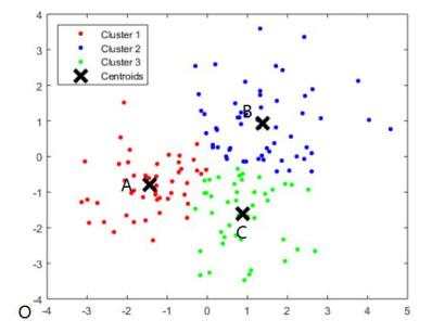
Figure 2 Centroids A, B, C location |
Full size|PPT slide
The total distance from demand dots to A cluster centroid is 58.9621 km, the distance from demand dots to cluster B centroid is 115.1753 km, the distance from demand dots to cluster C centroid is 61.5390. The sum of all the dots to its centroids distances is 235.6764 km. So the flight distance of drone is double that distance, which is 471.3528 km.
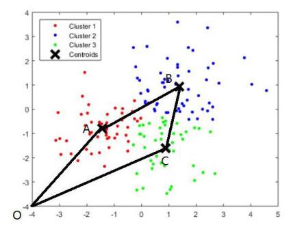
The coordination of centroids and supply center is as following: , , , . We solve this simple TSP problem by enumerating. Distance matrix is as following: The shortest distance is 15.4252, which is route or .
The distance of route : 15.4252 *
The distance of route : 16.4452
The distance of route : 18.4772
The distance of route : 16.4452
The distance of route : 18.4772
The distance of route : 15.4252 *
Figure 3 The TSP route with warehouse at O location |
Full size|PPT slide
5 TSP Method Case
The notations of all the parameter are as following:
stands for the total distance of TSP.
constant represents the distance between city and city .
The variable stands for whether the route from city tocity is taken by the solution.
The truck route starts from the distribution center.
The truck route ends at the distribution center.
is the total number of cities that needs to be visited. or means distribution center when it serves as the deliverystarting point and ending point separately.
The mathematical model can be seen as following.
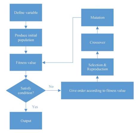
The equation (5.1) is the shortest distance objective. The equation (5.2) indicates that the truck is started from the distribution center. The equation (5.3) indicates that the truck running route is ending at distribution center. The sub-route elimination equation is (5.4). The equation (5.4) means the is visited only once. The equation (5.6) means that route start from has only one destination. The condition (5.7) is about value constraints of the variable. The equation (5.8) is used to show the non-negative attribute of . The TSP problem is NP-hard problem, so we use genetic algorithm to do the calculation and solve the TSP problem. The process of genetic algorithm is shown in Figure 4.
Figure 4 The process of genetic algorithm solve TSP |
Full size|PPT slide
The total number of city needs to be visited is 151, thus we have
. The coordination of depot and demand spots have been givenas
and
. The following Algorithms 1–9 is the code ofTSP solving. The selection operation is set in Algorithm 1
[12].
Algorithm 1 Selection operation
function seln=sel()
seln=zeros(2,1);
choose two individual from the population, better not choose same individual of two actions
for =1:2
=rand; generate a random number
prand=;
;
while
;
end
seln; Select the serial number
if &&==seln() if they are the same, select again
=rand; generate a random number
=rand; prand=;
;
while
;
end
end
end
end
The crossover operation of genetic algorithm is done in Algorithm 2.
Algorithm 2 Crossover operator
function scro=cro(,seln,)
bn=size();
pcc=pro(); decide whether to do crossover according to crossover rate, if pcc equal 1, then we will do crossover, if pcc equals 0, then we will not do crossover.
scro(1,:)=(seln(1),:);
scro(2,:)=(seln(2),:);
if pcc==
c1=round(rand*())+1; generate a crossover position among the range .
c2=round(rand*())+1;
chb1=min(c1,c2);
chb2=max(c1,c2);
middle=scro(1,chb1+1:chb2);
scro(1,chb1+1:chb2)=scro(2,chb1+1:chb2);
scro(2,chb1+1:chb2)=middle;
for =1:chb1
while find(scro(1,chb1+1:chb2)==scro())
zhi=find(scro(1,chb1+1:chb2)==scro());
=scro(2,chb1+zhi);
scro()=;
end
while find(scro(2,chb1+1:chb2)==scro())
zhi=find(scro(2,chb1+1:chb2)==scro());
y=scro(1,chb1+zhi);
scro(;
end
end
for =chb2+1:bn
while find(scro(1,1:chb2)==scro())
zhi=logical(scro(1,1:chb2)==scro());
=scro(2,zhi);
scro(;
end
while find(scro(2,1:chb2)==scro())
zhi=logical(scro(2,1:chb2)==scro());
=scro(1,zhi);
scro(;
end
end
end
end
The mutation operation is shown in algorithm 3 mutation operator.
Algorithm 3 Mutation operator
function snnew=mut(snew, pm)
bn=size(snew,2);
snnew=snew;
pmm=pro(pm); decide whether to do mutation operator accordingto mutation rate. If pmm=1, then mutation is done. Otherwise, nothing will be done.
if pmm==1
c1=round(rand*())+1; generate a random mutation position among the range of [].
c2=round(rand*())+1;
chb1=min(c1,c2);
chb2=max(c1,c2);
=snew(chb1+1:chb2);
snnew(chb1+1:chb2)=fliplr();
end
end
The city location coordination is set in Algorithm 4.
Algorithm 4 Pseudo-code for city location coordination
function [DLn,cityn]=tsp()
DLn=zeros();
if ==cityNum city151=[warehouse;all demand points];
for
for
DLn;
end
end
city =city151;
end
The fitness function calculation code is shown Algorithm 5, thefitness value is the shorter the distance the better.
Algorithm 5 Fitness function
function =CalDist(dislist, )
Distan ;
=size();
for
DistanV=DistanV+dislist();
end
DistanV=DistanV+dislist();
=DistanV;
end
The mutation process is an important of producing new solution. The algorithm 6 show the decision process of carrying on mutation or not.
Algorithm 6 Decide whether to do mutation action bychecking mutation rate.
function pcc=pro()
test(1:100)=0;
l=round(100*);
test(1:l)=1;
=round(rand*99)+1;
pcc=test();
end
The objective function value is calculated in Algorithm 7, which is the shortest distance.
Algorithm 7 Objective function
function =objf(, dislist)
inn=size(); %read population size
=zeros(inn,1);
for =1:inn
=CalDist(dislist, ,:)); calculate the function value, which is fitness value.
end
; get reciprocal of distance
calculate individual selected rate according to its fitness value.fsum=0;
for =1:inn
; the higher fitness value, the higher been chosen rate
end
ps=zeros(inn,1);
for =1:inn
;
end
calculate accumulate rate
p=zeros(inn,1);
;
for =2:inn
;
end
;
end
Algorithm 8 is the main function. The max generation is set 1500, the crossover rate is set to 0.8, the mutation rate is set to 0.08. The population size is 30.
Algorithm 8 function
CityNum=151;
[dislist,Clist]=(CityNum);
inn=30; original population size
gnmax=1500; max generation
=0.8; crossover rate
=0.08; mutation rate
produce original population
=zeros(inn,CityNum);
for =1:inn
=randperm(CityNum);
end
=objf(, dislist);
;
ymean=zeros();
ymax=zeros();
xmax=zeros(inn,CityNum);
scnew=zeros(inn,CityNum);
smnew=zeros(inn,CityNum);
while gnmax+1
for =1:2:inn
seln=sel(); selection operator
scro=cro(,seln,); crossover operator
scnew(,:)=scro(1,:);
scnew(,:)=scro(2,:);
smnew(,:)=mut(scnew(,:),pm); mutation operator
smnew(,:)=mut(scnew(,:),pm);
end
=smnew; generate new population
[]=objf(,dislist); calculate the new fitness value
record the current best and average fitness value
[fmax,nmax]=max();
ymean(gn)=1000/mean();
ymax(gn)=1000/fmax;
record current generation best individual
(nmax,:);
max(gn,:)=;
drawTSP(Clist,,ymax(), ,0);
;
end
;
;
figure(2);
plot(ymax,'');hold on;
plot(ymean,'');grid;
title('Searching Process');
legend('Best solution','Average solution');
fprintf('The shortest distance got by genetic algorithm: %.2fn',minymax);
fprintf('The shortest route generated by genetic algorithm');
disp(xmax(index,:));
end
The algorithm 9 is set to draw pictures of the TSP running result.
Algorithm 9 Draw picture
function drawTSP(Clist,BSF,bsf,)
CityNum=size(Clist,1);
for =1:CityNum
plot([Clist(BSF(),1),Clist(BSF(+1),1)], [Clist(BSF(),2), Clist(BSF(+1),2)],'ms',
'LineWidth',2,'MarkerEdgeColor','','MarkerFaceColor','');
text(Clist(BSF(),1),Clist(BSF(),2), [' ',int2str(BSF())]);
text(Clist(BSF(),1),Clist(BSF(),2), [' ',int2str(BSF())]);
hold on;
end
plot([Clist(BSF(CityNum),1), Clist(BSF(1),1)], [Clist(BSF(CityNum),2), Clist(BSF(1),2)], 'ms', 'LineWidth', 2,'MarkerEdgeColor', '', 'MarkerFaceColor', '');
title([num2str(CityNum), 'cities TSP']);
if ==0&&CityNum =10
text(5,5, ['The No.',int2str(), 'generation', 'The shortest distance is',num2str(bsf)]);
else
text(5,5, ['The final searching result: The shortest distance',num2str(bsf), 'got at No.',num2str(p), 'generation']);
end
if CityNum==10
if ==0
text(0,0,['At No. ',int2str(p), 'generation', 'The shortest distance is', num2str(bsf)]);
else
text(0,0,['The final searching process result: The shortest distance is', num2str(bsf), 'got at', num2str(), 'generation']);
end
end
hold off;
pause(0.05);
end
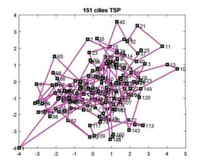
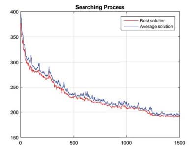
The running environment is as following. Operating system: Windows10 Enterprise 64 bytes; CPU: Intel Core i7-5500U @ 2.40GHz dual coreprocessor; memory: 8 GB. The running result is shown as following.The shortest distance got by genetic algorithm is 189.69. Theshortest route can be seen in Figure 5. The searching process can beseen in Figure 6.
Figure 5 The 151 cities TSP solution gotby genetic algorithm |
Full size|PPT slide
Figure 6 The TSP searching process |
Full size|PPT slide
6 Result and Analysis
6.1 One Drone Case
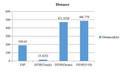
The truck running distance of DTSP method saves 91.87, the truckrunning distance is shortened from 189.69 km to 15.4252 km. Theflight distance is longer than the TSP method, because the drone isdeliverying one parcel at a time. The detail can be seen in Figure 7.
Figure 7 The running distance of TSP andDTSP method |
Full size|PPT slide
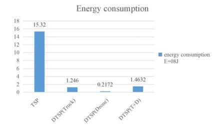
According to research of Sergio Ferrandez, et al.[13], thetruck's energy is J, which is J, we can get J/km by calculation. The drones' speed is 70km/h, the truck's speed is 35 km/h. The drone's energy consumptionis 896 Joules per second and fly at 70 km/h. The drone's flightdistance is 471.3528 km. We can get 6.7336 h for one drone to flyover, which is s. Then we can get the energyconsumption of drone, which is J. The energy consumption of traditionalTSP method is J. The energy consumption of thedrone TSP method is only J, which accounts thetraditional TSP method 9.55. The DTSP method saves 90.45 ofenergy. The drone's energy consumption is tiny. The content can beseen in Figure 8.
Figure 8 The energy consumption of TSP and DTSP method |
Full size|PPT slide
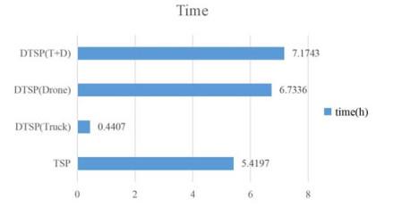
The delivery time of DTSP method delivering is 7.1743 h, thetraditional TSP method is 5.4197 h. The DTSP way of delivering uses132.37 more time than the traditional TSP method, which meansa 32.37 adding in time aspect. The truck delivery time isdropping from 5.4197 h to 0.4407 h. The content can be seen in Figure 9.
Figure 9 The running time of TSP and DTSP method |
Full size|PPT slide
Table 1 is the data of the comparison of TSP and DTSP method indistance, Energy consumption and time in one drone case.
Table 1 The comparison of two ways of delivering in one drone case |
| Way of delivery | TSP | DTSP (Truck) | DTSP (Drone) | DTSP (Truck+Drone) |
| Distance | 189.6900 km | 15.4252 km | 471.3528 km | 486.778 km |
| Energy consumption | 1.532×10⁹ J | 1.246×10⁸ J | 2.172×10⁷ J | 1.4632×10⁸ J |
| time | 5.4197 h | 0.4407 h | 6.7336 h | 7.1743 h |
6.2 Multi-Drone Case
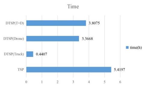
Two drone case is used as example. The total distance and energyconsumption will stay the same. But the delivery time can beshorten a lot. The more drone the less time consumption is obvious.The advantage of drones can be more obvious when there aremultiple-drone cases. But there is an limitation of truck load. Herewe use two drones as an example. If there are two drones on thetruck. The distribution time will save 29.75, the time will beshorten to 3.8075 hour from 5.4197 hour. The data can be seen in Figure 10.
Figure 10 The running time of TSP and DTSP method |
Full size|PPT slide
Table 2 shows the data of the comparison of TSP and DTSP method in distance, energy consumption and time in two drones case.
Table 2 The comparison of two ways of delivering in two drone case |
| Way of delivery | TSP | DTSP (Truck) | DTSP (Drone) | DTSP (Truck+Drone) |
| Distance | 189.6900 km | 15.4252 km | 471.3528 km | 486.778 km |
| Energy consumption | 1.532×10⁹ J | 1.246×10⁸ J | 2.172×10⁷ J | 1.4632×10⁸ J |
| time | 5.4197 h | 0.4407 h | 3.3668 h | 3.8075 h |
7 Discussion and Future Research
Recent practice of small parcel delivery by Amazon, JD, Google andDHL has shown the potential of drones for small parcel delivery.While a lot of papers focus on mechanical aspect of drone, thisarticle studies its operational problem. In particular we build amodel of drone and truck in tandem system. We bring out dronetraveling salesman problem. We compare our method with thetraditional TSP method. The result shows our new method hasadvantages in distance of truck running, energy consuming and timeusage. All the data give us a picture of the great potential indrone parcel delivery. Due to the limit number of drone usagepractice, we are in shortage of cost data. We have limits on costcalculation. In the future, the cost calculation and comparison willbe the research direction.
{{custom_sec.title}}
{{custom_sec.title}}
{{custom_sec.content}}
 PDF(396 KB)

 Figure 1 Demand point clustering
 Table 1 The comparison of two ways of delivering in one drone case


