1 Introduction and Literature Review
Since 2013, the proportion of service industries in the national economy has exceeded the manufacturing, which has become the largest industries in China. Just as the advanced manufacturing and strategic emerging industries, service industries especially the modern service industries are becoming the important symbols of China's economic development towards middle and high level. However, unlike the output of manufacturing, the output of service industries has the characteristics of invisibility and high degree of difference. Besides, the producer services have the characteristics of intermediate input, knowledge intensive and high entry barriers. These characteristics mean that once element allocation distortions, the service industries will also face the predicament of overcapacity. Therefore, the scientific measurement of element input and productivity difference in service industries has important theoretical and practical significance for improving the quality and efficiency of the supply side.
1.1 Review of Capital Input
In the estimation of element input, measurement of capital input is relatively complex and difficult. It is not only because of the heterogeneity of different categories of assets, made it difficult to compare and aggregation, but also and more importantly, the understanding of capital contribution to production has gone through a deepening process. As the official statistical authority in the world, the System of National Accounts (SNA) has not been officially confirmed the concept of productive capital stock and capital services until the latest revised edition in 2008. Then, it introduced how to calculate and measure the contribution to output of capital.
Prior to this, foreign scholars have applied the concept of capital services to the related fields. In 1963, Jorgenson
[1] took the lead in constructing the capital flow accounting framework based on Goldsmith
[2]'s capital stock theory, and made an empirical analysis based on the actual data of the United States
[3-5]. In 1990s, the theory of capital accounting was further improved and developed by Hulten
[6, 7], et al. At the beginning of the 21st century, the capital service theory was gradually maturing with the impetus of Diewert, et al.
[8-10]. Scholars begins to use this system to conduct empirical research on different countries, for example, Schreyer
[11] analyzed the size of capital input in the United Kingdom, Italy, Germany and other OECD countries; Erumban
[12] analyzed capital productivity in European Union and American; Wallis
[13] estimated the time series of capital service in British; Inklaar
[14] compared the capital input at different rates of return.
At present, most of the researches of capital input in China are based on the value measurement of capital stock. There is very little literature based on the framework of capital services. Sun and Ren
[15-17] carried out empirical research on China's capital services using geometric model for the first time; Ye
[18], Cai
[19] took the lead in using hyperbolic model to study the scale of capital investment in China; Cao
[20] applied the framework of capital services to the provincial scope; Xi and Xu
[21] measured the input of R & D capital services in China; Ye
[22] estimated the level of capital services in the trade and circulation industry. Generally speaking, the current research of capital stock and flow based on the definition of productivity is still rare in China.
1.2 Review of Service Industries Productivity
By concern for economic growth, there are many studies on the productivity of services at home and abroad. Yang and Su
[23] studied the efficiency of the service industry in the East, middle and West China using the SFA parameter method in 1993–2007; Jiang and Gu
[24] calculated the productivities of eight service industries in China in 1978–2006; Huang and Huang
[25] also used the SFA model to analyze the regional differences in the productivity of transport storage and communications industries, finance and insurance, wholesale and retail trade, and catering industries in 1993–2008. Because the parameter method depends on the exact form of the production function in estimation, it is usually impossible to avoid the problem of setting bias. Besides, due to the existence of incomplete competition such as monopoly pricing, the assumptions of these models are difficult to meet.
As the representative of the nonparametric method, the data envelopment analysis (DEA) does not seek the specific form of production function, and with endogenous weight, it does not need to make assumptions about market competition, so it is more and more popular in the research of productivity. Liu and Zhang
[26] measured the total factor productivity changes in the service sector of China's 28 provinces and cities by using the non-parametric Malmquist index method in 1978–2007. Pang and Deng
[27] used 1998–2012 provincial panel data to measure the productivity and growth rate of service industry. Wang and Teng
[28] took the environment factor into consideration, calculated the total factor productivity changes in 31 provinces and cities in 2000–2012. In general, these studies are deeply and systematically, and with high reference value. However, the traditional DEA model ignores the statistical test, and the significant level of productivity estimation is not given, thus it is lack of accuracy and robustness.
On the basis of these studies, this paper will enrich the existing literature in the following two aspects: Firstly, according to the framework of capital services, we use hyperbolic model to measure the capital input in China's 36 service sectors in 2003–2015. Secondly, we use the four stage Bootstrap-DEA model to control the impact of external factors, calculate the productivities and its confidence intervals of the 36 service sectors. Finally, according to the calculation results, we compare the difference of the productivities in these service sectors.
2 Productive Capital Stock Measurement Framework
Capital service is an efficiency concept expressed in the form of flow, which is based on the concept of productive capital stock. In the same production cycle, capital services is a fixed proportion of productive capital stock, so in the productivity accounting, the productive capital stock growth index is the same as capital service growth index.
Productive capital stock is different from wealthy capital stock. The former is based on the efficiency of capital goods, which embodies the production capacity of capital. The latter is based on the value of capital goods, which embodies the wealth of capital. Taking a one-year-old light bulb as an example, the wealthy capital stock reflects its market value, and the productive capital stock reflects its productivity. Obviously, as far as the light bulb is concerned, its productivity is no different from that of the new bulb, but its value is far from the new bulb. Therefore, in this sense, the traditional wealthy capital stock does not apply to the measurement of capital output efficiency.
2.1 Aggregation Weights of the Same Type of Assets
Because the assets are different in age, they cannot be directly aggregated even belongs to the same type. The aggregate weights should reflect the change of assets with age. The change of assets with age is either embodies the value change, or embodies the efficiency change. The former is named age-price coefficient, and the latter is named the age-efficiency coefficient.
The common models of the age-efficiency coefficient are the single carriage model, the linear decline model, the geometric model and the hyperbolic model. Single carriage model suggests that the asset efficiency is constant, which does not change with time. The linear decline model suggests that the assets efficiency decreases linearly with time, and the slope is negative. The main difference between the geometric model and the hyperbolic model is that in the initial stage of the capital investment, the geometric mode decreases rapidly, and the hyperbolic mode decreases slowly. The example of the bulb shows that the hyperbolic decline model is more in line with the actual situation when describing the asset efficiency change. The hyperbolic model can be expressed as
In the equation, represents the service life of the asset, represents the actual age of the asset, and is a parameter of efficiency decreasing. When the age-efficiency coefficient follows a hyperbolic model, it indicates that the asset's efficiency presents a decreasing characteristic in hyperbolic form over time.
2.2 Productive Capital Stock in a Specific Type
Through the age-efficiency coefficient (between 01), the new and old assets from the same type of economy, can be unified into the initial state and summarized. The Perpetual Inventory Method (PIM) is used to aggregate the same type of capital stock. It should be noted that, we also use the PIM method to summarize the wealthy capital stock, but the weights in wealthy capital stock are age-price coefficient, not the age-efficiency coefficient here. The aggregation equation for a specific category of productive capital stock is
In the equation, represents the asset's productive capital stock at year , and represents the investment of -year-old asset at the year of , is an integrated coefficient of age-efficiency.
2.3 Aggregation Weights of Different Types of Assets
In the collection of different types of assets, it is necessary to take the capital return share as the weight of the asset. Capital return is the product of user cost and productive capital stock. The user cost is equal to the price of capital services. Under the condition of perfect competitive market, the user's cost is the rental price of the specific asset in a given period. In reality, most of the asset rental prices are not from the effective market, so the observed rental price is not a good reflection to the current value of capital services. The equation for calculating the user cost in practice is
In the equation, represents the user cost of asset in year . represents the return of asset in year . represents the depreciation rate of assets in year . and , respectively, represent the prices of asset in the year of and .
2.4 Aggregating Different Types of Productive Capital Stock
The accumulation of productive capital stock of different types usually takes the form of index. The axiomatic approach requires that, good index should satisfy the tests of identity test, commensurability test and time reversal test. Fisher index and Tornqvist index are the excellent indexes which satisfy this series of tests. Stochastic approach holds that the calculation of index is similar to estimating parameters, we can choose index by estimating its standard error. According to this standard, Tornqvist index is better than Fisher index. Based on the above, Tornqvist index is used to summarize the productive capital stock here.
3 Four Stages Bootstrap-DEA Productivity Model
DEA model is one of the most important methods to measure the relative efficiency of decision making unit (DMU), which is based on the efficiency theory of Farrell
[29]. It mainly uses mathematical programming tools to build an effective production frontier, and then compares the effectiveness of decision making units with the effective production frontier.
3.1 Classical DEA Model
The basic model of DEA can be divided into two types: The constant returns to scale (CRS) and the variable returns to scale (VRS). In 1978, Charnes, Cooper
Rhodes
[30] first proposed the constant scale DEA model, referred to as CCR model. Assuming that there are
decision making units in the production system, the input is denoted as
, and the output is denoted as
, then the production efficiency of the
th decision making unit, which is
, can be solved by the following linear programming:
In the equation,
means weight parameters:
and
are slack variables, which indicates the space of inputs and outputs that can be improved;
and
are the input and output when decision making units are valid. In 1984, Banker, Charnes and Cooper
[31] added the constraint of
to the upper equation, that is, the BCC model. The CCR model and BCC model are input oriented models, which measure the redundancy of inputs under the premise of fixed output. The range of the efficiency value is 0
1.The lower the value, the lower the relative efficiency.
3.2 Four Stages DEA Model
The defect of the classical DEA model is that it does not take into account the influence of external environmental factors and random factors in the redundancy. The redundant information is the difference between the actual input and the theoretical input, which is not negative. Due to the general regression model will lead to the bias of the estimated parameters to zero, we need to use the Tobit regression model which can deal with the problem of data truncation. This process is divided into four stages:
In the first stage, the classical DEA model (BCC model or CCR model) is used to calculate the redundancy of each decision making unit.
In the second stage, the Tobit regression model is constructed with the input redundancy as the dependent variable and the external environmental factors as independent variables:
In the formula, is the redundancy of input in the th service sector, is an exogenous environmental disturbance variable, is a vector of coefficients to be estimated, is a random error term. The estimated coefficient reflects the correlation between exogenous factors and input redundancy. If the value is negative, indicating that the increase of exogenous variables is conducive to reduce the input redundancy, thereby reducing waste or negative output.
In the third stage, the input of each decision making unit are adjusted by the regression result of limited dependent variable. It increases the unit input with good external environment condition, and reduces the unit input with weak external environment, to make all decision making units in the same external environment. The adjustment equation is
In the equation, represents fitting value of the redundancy of input in the th service sector, represents the input in the th service sector. means the adjusted input, that is, the input after eliminating the impact of external environmental factors.
In the fourth stage, the adjusted input data is used as the initialinput of each unit, and the output remains unchanged. Theefficiency of each service sector is recalculated by using theclassical DEA model.
3.3 Bootstrap-DEA Model
Although without interference of external factors, the ordinary DEA method cannot estimate the asymptotic distribution of the estimated efficiency, and cannot give the confidence interval and the significance level of the estimated value. In order to solve these problems, Simar and Wilson
[32, 33] proposed the Bootstrap-DEA model. The idea is to extract pseudo samples through replacement sampling. After a certain number of repetitions, the empirical density function in pseudo sample can be obtained. Then the Monte Carlo method is used to correct the parameter deviation and construct the confidence interval. The specific process is:
1) According to the original output and the adjusted input of the four stage DEA model, the classical DEA model is used to calculate the initial efficiency of each service sector.
2) Taking the initial efficiency as population, samples of size are obtained by replacement sampling. Then smooth the data in the samples, obtain . The smoothing equation is
In the equation, is the bandwidth or smoothing parameter, and is random error of standard normal distribution.
3) Using efficiency value after smoothing to adjust original input data .
4) According to the adjusted input and original output to re-estimate the efficiency value .
5) Repeat the process 2)4), iterate times, we can get the statistical distribution of the efficiency value and correct the error:
Error of efficiency value is: bias;
Corrected efficiency value is: .
4 Data and Parameter Selection
4.1 Data Processing
4.1.1 Capital Investment
The basic data of capital input is the annual investment data of service sectors. The relevant statistical indicators are "total investment in fixed assets in the whole country" and "gross capital formation". The former considers the difference of different assets, which can be further subdivided into construction and installation, purchase of equipment and instruments, and other expenses. The latter is directly from the constituent items of GDP accounting, which is more suitable for the analysis of capital services. However, the data of gross capital formation in subdivision industries can only be seen in a few years. In contrast, "China Fixed Assets Investment Statistics Yearbook" published the data of total investment in fixed assets in types of asset regularly, so we will choose "total investment in fixed assets" indicator in our study.
4.1.2 Labor Input
In the current official statistics, there are two sets of labor data in service sector, namely, "the staff number" in the China Statistical Yearbook and "the quantity of employment" in the China Labor Statistical Yearbook. Statistical standard of "the staff number" is the number of official workers. In terms of the labor input consumed by production, it is not comprehensive enough. In contrast, "the quantity of employment" can be more accurately to reflect the actual employment situation, so we select "the quantity of employment" as labor input indicator.
4.1.3 Output Data
The output variable is the value-added in service sectors. At present, China Statistical Yearbook publishes value-added data of 14 service sectors annually, more detailed sectors' data only given by the Chinese Input-Output Table. The research period of this study is 2003–2015, in which the data of 36 service sectors in 2007 and in 2012 are directly taken from China's input-output table, and the data of 36 service sectors in 2005 and in 2010 are directly taken from the input-output extension tables. For the remaining years, the value-added of service sectors provided by the China Statistical Yearbook is decomposed by the proportion structure of the adjacent years.
4.1.4 External Environment Variables
To estimate the productivity of each sector, we need to control the influence of external environment. In this paper, three variables, "average education level", "average weekly working time" and "average wage", are taken as the external variables of each decision making unit. Among them, the average level of education is converted by years of schooling. The average wage is revised according to the average wage index and take 2003 as the base year. The original data come from the annual "China Labor Statistical Yearbook".
4.1.5 Price Index
In order to eliminate the impact of price fluctuation, it is necessary to deflate the indices of "total investment in fixed assets" and "value-added in service sectors". "China Statistical Yearbook" provides the fixed asset investment price indices in assets types. We take 2003 as the base year, sequentially revise the investment sequence of these three assets in 2003–2015. "China Statistical Yearbook" also provides the GDP deflator in sectors for the past years. We still take 2003 as the base year, sequentially revise the value-added of service sectors in 2003–2015.
4.2 Parameter Selection
The calculation of capital inputs also requires the following parameters:
1) Age-efficiency coefficient () and efficiency decreasing parameter . The life span of different types of assets is different, the decline degree of efficiency is different in every year, so the impact on capital accumulation is also different. Referring to the nature of different assets and previous research experience, we set the life parameters of equipment and instruments for 15 years, construction and installation for 40 years, and other expenses for 20 years. Similarly, for efficiency decreasing parameter , we set equipment and instruments for 0.5, construction and installation for 0.75, and other expenses for 0.61.
1 In general, the longer the use of assets, the higher the value of . We mainly refer to the value standard from the Australian Bureau of Statistics.
2) Initial capital stock (). In each period there are assets to enter and withdraw from the economic system. In theory, investment flows can be traced forward indefinitely. Restricted by various factors, we can only extract a certain period of time to study, so we need to set the initial value. Under the assumption that the initial stock growth rate is equal to the initial investment growth rate, the formula can be deduced as . In the formula, represents the initial investment flows, represents investment growth rate, represents depreciation rate.
3) Return on assets . The rate of return on assets can be endogenous or exogenous. Endogenous returns are based on the equilibrium calculation of macroeconomic accounting, which requires not only new data, but also are affected by data sources and data quality. In different years, the volatility of the return on assets between industries is large, and even leads to negative value. In order to eliminate the impact of extreme values, we use exogenous method to determine the rate of return on assets. Reference to the bank's medium and long-term loan interest rates, we eventually set the return on fixed assets of 5.
4) Depreciation rate . Similar to the rate of return, there are two ways to determine the depreciation rate. In the geometric model, the depreciation rate is usually determined exogenously, or based on historical accounting information such as fixed assets' net value. Different from the above two approaches, the depreciation rate can be deduced from the age-efficiency coefficient in this paper. It belongs to the endogenous method, but does not need additional information. In addition, the depreciation rate obtained by this method can be directly used to calculate the wealthy capital stock, which is easy to compare with the productive capital stock under the framework of capital services.
4.3 Industry Classification
According to the latest revision of National Economic Industries Classification (GB/T4754-2011), service industry consists of 46 two digit sectors. Due to the adjustment of statistical caliber in some years, we unified the "repair industry" into "other services"; combine "computer services" and "software" into "computer services and software"; combine "wholesale" and "retail" as "wholesale and retail"; combined "banking" and "securities" into "banking and securities". We also combine the "international organization" and "grassroots autonomous organizations, mass organizations, social organizations and other members of the organization", "the CPPCC, democratic parties", "Chinese party" and "national institutions" into "public management and social organization". Finally, the 36 service sectors are formed, with the corresponding codes and sector names shown in Table 1.
Table 1 Classification and coding of service sectors |
| No | Sector | | No | Sector | | No | Sector |
| 1 | Railway transportation | | 13 | Catering | | 25 | Resident service dustries |
| 2 | Road transport dustries | 14 | Banking securities | 26 | Other services |
| 3 | Water transportation dustries | 15 | Insurance industries | 27 | Education |
| 4 | Air transport dustries | 16 | Real estate | 28 | Hygiene |
| 5 | Pipeline transportation | 17 | Leasing industries | 29 | Social security dustries |
| 6 | Handling and other transport services | 18 | Business services | 30 | Social welfare dustries |
| 7 | Warehousing dustries | 19 | Research and experimental development | 31 | Press and publication |
| 8 | Postal industries | 20 | Professional technical service | 32 | Radio, television, film and video industries |
| 9 | Telecommunications and other information transmission services | 21 | Science and technology exchange and service promotion | 33 | Culture and art |
| 10 | Computer services and software | 22 | Water conservancy management | 34 | Sports |
| 11 | Wholesale and retail trade | 23 | Environmental management industries | 35 | Entertainment |
| 12 | Lodging industries | 24 | Public facilities management | 36 | Public management and social organization |
5 Empirical Analysis Results
5.1 Productive Capital Stock
According to the latest SNA standard, capital input is calculated onthe basis of productive capital stock. Table 2 gives the calculationresults of the productive capital stock of the 36 service sectors.On average, the service sectors which have the higher productivecapital stock are the real estate industry, road transport, telecommunications, public management and social organizations. Theservice sectors which have relatively small productive capital stockare leasing, social security, insurance, social welfare, and so on.
Table 2 Productive and wealthy capital stock in service sectors (2003–2015)2 unit: 0.1 billion yuan |
| sectors | Productive Capital Stock | | Wealthy Capital Stock |
| 2003 | 2006 | 2009 | 2012 | 2015 | 2003 | 2006 | 2009 | 2012 | 2015 |
| No.1 | 3640 | 7206 | 17528 | 31006 | 40743 | | 2879 | 5894 | 14927 | 25927 | 33991 |
| No.2 | 32982 | 49126 | 71533 | 104584 | 132026 | 26653 | 39995 | 58082 | 84665 | 106939 |
| No.3 | 3944 | 5936 | 8906 | 12728 | 15767 | 2904 | 4512 | 6848 | 9723 | 12072 |
| No.4 | 1954 | 2822 | 4088 | 5732 | 7180 | 1283 | 1926 | 2845 | 4059 | 5153 |
| No.5 | 386 | 611 | 813 | 1090 | 1438 | 312 | 493 | 636 | 840 | 1121 |
| No.6 | 176 | 315 | 653 | 1662 | 2525 | 158 | 276 | 566 | 1446 | 2200 |
| No.7 | 498 | 1223 | 3528 | 8834 | 12958 | 430 | 1071 | 3132 | 7778 | 11396 |
| No.8 | 216 | 272 | 316 | 412 | 504 | 167 | 205 | 230 | 303 | 374 |
| No.9 | 28089 | 31745 | 35026 | 35924 | 38066 | 15112 | 17099 | 18605 | 18386 | 19370 |
| No.10 | 109 | 313 | 769 | 2172 | 3443 | 94 | 274 | 667 | 1907 | 3024 |
| No.11 | 3991 | 8011 | 15946 | 31656 | 44710 | 3368 | 6847 | 13661 | 27117 | 38381 |
| No.12 | 965 | 2203 | 5052 | 11266 | 15710 | 837 | 1938 | 4448 | 9907 | 13777 |
| No.13 | 563 | 1145 | 2554 | 4853 | 6564 | 457 | 958 | 2188 | 4141 | 5598 |
| No.14 | 420 | 675 | 1206 | 2443 | 3460 | 314 | 512 | 948 | 2008 | 2882 |
| No.15 | 20 | 40 | 69 | 212 | 292 | 14 | 30 | 53 | 183 | 253 |
| No.16 | 66157 | 112940 | 196675 | 355129 | 476397 | 53971 | 93240 | 163612 | 298315 | 400960 |
| No.17 | 10 | 49 | 200 | 610 | 974 | 8 | 42 | 171 | 500 | 801 |
| No.18 | 1046 | 2348 | 5352 | 12476 | 18067 | 904 | 2047 | 4687 | 10967 | 15885 |
| No.19 | 995 | 1603 | 2499 | 3982 | 5202 | 770 | 1259 | 1965 | 3165 | 4162 |
| No.20 | 209 | 475 | 988 | 2263 | 3325 | 179 | 407 | 844 | 1950 | 2867 |
| No.21 | 123 | 298 | 658 | 1613 | 2530 | 107 | 262 | 577 | 1417 | 2226 |
| No.22 | 3535 | 5736 | 9420 | 16863 | 22450 | 2923 | 4768 | 7872 | 14244 | 18990 |
| No.23 | 1330 | 2198 | 4148 | 7040 | 9127 | 1044 | 1759 | 3422 | 5815 | 7545 |
| No.24 | 18032 | 31201 | 56250 | 99453 | 135209 | 14214 | 25351 | 46693 | 83261 | 113899 |
| No.25 | 197 | 449 | 979 | 2348 | 3407 | 172 | 395 | 859 | 2071 | 3007 |
| No.26 | 138 | 260 | 560 | 1787 | 2508 | 100 | 196 | 450 | 1556 | 2179 |
| No.27 | 15020 | 20120 | 25918 | 33901 | 41165 | 11611 | 15611 | 19925 | 25962 | 31594 |
| No.28 | 1996 | 3409 | 5778 | 9674 | 12762 | 1596 | 2763 | 4718 | 7958 | 10532 |
| No.29 | 11 | 40 | 133 | 488 | 683 | 9 | 36 | 121 | 448 | 623 |
| No.30 | 56 | 138 | 410 | 1022 | 1567 | 50 | 125 | 375 | 924 | 1417 |
| No.31 | 121 | 174 | 291 | 420 | 543 | 88 | 129 | 227 | 330 | 433 |
| No.32 | 354 | 604 | 953 | 1390 | 1848 | 284 | 490 | 765 | 1102 | 1478 |
| No.33 | 480 | 1010 | 2229 | 5158 | 7402 | 422 | 887 | 1962 | 4561 | 6535 |
| No.34 | 616 | 1050 | 1777 | 3031 | 4103 | 489 | 855 | 1468 | 2533 | 3450 |
| No.35 | 605 | 1167 | 2418 | 4706 | 6366 | 514 | 998 | 2086 | 4027 | 5438 |
| No.36 | 21699 | 27786 | 34806 | 44592 | 52283 | 15023 | 19632 | 24856 | 32663 | 38646 |
2This paper only shows the total capital stock, capital stock in detail asset types can be obtained from the author.
From the view of capital growth, the service sectors with a high growth rate includes the leasing sectors, computer and software service, science and technology promotion sector, business service, culture and arts. The service sectors with a low growth rate includes public management and social organization, education, air transport industries, press and publishing industries and so on. It can be found that there is a negative correlation between the capital stock and the growth rate in most industries. The sectors with less capital stock tend to develop rapidly, while the sectors with higher capital stock tend to develop slowly.
5.2 Wealthy Capital Stock
Most of the domestic literature in capital input is to estimate the wealthy capital stock. For the convenience of comparison, this paper deduces the corresponding depreciation rate according to the age-efficiency parameters, and calculates the wealthy capital stock, the results are shown in Table 2. From the calculation results, the productive capital stock of each sector is significantly higher than its wealthy capital stock. The results indicate that the wealthy capital stock underestimates the actual size of capital services in production, and thus makes the calculation of factor productivity resulting in bias.
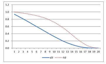
Specifically, productive capital stock is about 22 higher than wealthy capital stock in the research period on average. Sectors with larger difference in the two stocks usually have a higher growth rate. The main reason lies in the inconsistency between the age-efficiency coefficient and the age-price coefficient. Figure 1 shows that the efficiency coefficient and the price coefficient vary with time in the case of "other expenses" assets (with an average life span of 20 years). It can be found that the coefficient of efficiency is always higher than the coefficient of price in the life cycle. The efficiency coefficient is the base of the productive capital stock, and the price coefficient is the base of the wealthy capital stock. The former is higher than the latter, means that the market value of assets is always less than the capital services it can provide. Therefore, in terms of the whole economic system, the productive capital stock is higher than the wealthy capital stock.
Figure 1 Age-efficiency coefficient (h3) and age-price coefficient (d3) |
Full size|PPT slide
5.3 Factors Analysis of the External Environment Variables
In the process of calculating the efficiency scores of decision making units, we consider the input redundancy as the dependent variable, "the average wage", "weekly working hours" and "average education level" as the observable environment variables, analyze the factor effect of productivity in service sectors, the results are shown in Table 3.
Table 3 Tobit fitting results of external factors of service productivity |
| Variable | Intercept | weekly working hours | education level | average wage | ρ |
| initial value | 50.468610 | 0.000004730 | -0.691206 | -1.298071 | 0.7133 |
| adjusted value | 95.430050 | 0.000008283 | -1.318032 | -2.686845 | 0.7458 |
| the upper bound | 51.560710 | -0.000055509 | -2.772421 | -5.695489 | 0.8998 |
| the lower bound | 198.429400 | 0.000073434 | -0.683399 | -1.351283 | 0.6572 |
| Note: The regression uses 5 significance level; is the proportion of individual effect variance in total variance. |
The regression results show that the coefficient of "the average wage" is negative, and is in the 95 confidence interval, which means that "the average wage" has a significant negative impact on the input redundancy. The higher the average wage, the less redundancy in the industry, and the higher the sectoral productivity. Economic theory holds that the high average wage is the return on human capital with higher productivity. Therefore, a high level of wages indicates employees with a high level of technology and professional quality, which are usually necessary to maintain a higher productivity.
The coefficient of "the average education level" is significantlynegative and lower than the "average wage", indicating thatincreasing the education level of employees will also improve theinappropriate allocation of resources in service sectors, and willhave a significant positive effect on the productivity of serviceindustry. It is in line with expectation, because with the upgradingof service industry, the traditional extensive economic mode willgradually be replaced by the high-end, high efficiency productionmode. The latter must match employees with a higher level ofknowledge reserves and technical capabilities.
The coefficient of "weekly working hours" is small and notsignificant, which shows that the influence of average working timehas no practical significance on productivity. In general, longworking hours will effectively improve the level of output, butcannot be directly reflected in the productivity.
5.4 Sectoral Productivity Based on Four Stages Bootstrap-DEA
The four stages bootstrap-DEA model is used to calculate the sectoral productivity. Firstly, it is necessary to determine whether the CCR model or the BCC model is used to calculate the initial efficiency of the decision-making unit. According to the test results, the P values of the statistics are 0.507 for PCS and 0.701 for WCS, which cannot reject the null hypothesis of constant returns to scale. Therefore, we use the CCR model to calculate the initial value of productivity, and then use the four stages bootstrap-DEA to correct the productivity of the two stocks, the results are shown in Table 4.
Table 4 Average productivity in 36 service sectors (2003–2015) |
| | Based on Productive Capital Stock (PCS) | | Based on WCS | | Comparison |
| bias | adjusted | initial | lower | upper | bias | initial | PCS | WCS |
| No.1 | 0.0650 | 0.8830 | 0.9480 | 0.8645 | 0.9193 | | 0.8942 | 0.9558 | | 0.8350 | 0.8934 |
| No.2 | 0.0639 | 0.6377 | 0.7016 | 0.6083 | 0.6846 | 0.6764 | 0.7300 | 0.5803 | 0.6774 |
| No.3 | 0.0628 | 0.6460 | 0.7088 | 0.6196 | 0.6880 | 0.6533 | 0.7133 | 0.5377 | 0.6574 |
| No.4 | 0.0662 | 0.6625 | 0.7287 | 0.6320 | 0.7111 | 0.7751 | 0.8309 | 0.6027 | 0.7757 |
| No.5 | 0.1959 | 0.8041 | 1.0000 | 0.6609 | 1.0369 | 0.8142 | 1.0000 | 0.8277 | 0.8085 |
| No.6 | 0.0658 | 0.6615 | 0.7273 | 0.6312 | 0.7098 | 0.6629 | 0.7192 | 0.6013 | 0.6649 |
| No.7 | 0.0682 | 0.7110 | 0.7792 | 0.6825 | 0.7606 | 0.6315 | 0.7002 | 0.5713 | 0.6400 |
| No.8 | 0.0668 | 0.8510 | 0.9178 | 0.8296 | 0.8938 | 0.8943 | 0.9641 | 0.8108 | 0.8940 |
| No.9 | 0.1043 | 0.7217 | 0.8260 | 0.6597 | 0.8181 | 0.8587 | 1.0000 | 0.6261 | 0.8761 |
| No.10 | 0.0512 | 0.7680 | 0.8192 | 0.7569 | 0.7915 | 0.7613 | 0.8074 | 0.7032 | 0.7599 |
| No.11 | 0.1141 | 0.8859 | 1.0000 | 0.8244 | 0.9534 | 0.9131 | 1.0000 | 0.8362 | 0.9183 |
| No.12 | 0.0558 | 0.8453 | 0.9011 | 0.8336 | 0.8700 | 0.8374 | 0.8878 | 0.7765 | 0.8357 |
| No.13 | 0.0626 | 0.8791 | 0.9417 | 0.8627 | 0.9092 | 0.8841 | 0.9425 | 0.8272 | 0.8831 |
| No.14 | 0.0718 | 0.7409 | 0.8127 | 0.7096 | 0.7936 | 0.6874 | 0.7598 | 0.5824 | 0.6955 |
| No.15 | 0.0594 | 0.8926 | 0.9520 | 0.8800 | 0.9159 | 0.8933 | 0.9478 | 0.8266 | 0.8915 |
| No.16 | 0.1728 | 0.8272 | 1.0000 | 0.7077 | 0.9768 | 0.8559 | 1.0000 | 0.7766 | 0.8633 |
| No.17 | 0.0716 | 0.7236 | 0.7952 | 0.6928 | 0.7714 | 0.7034 | 0.7687 | 0.6117 | 0.7081 |
| No.18 | 0.0555 | 0.7602 | 0.8157 | 0.7448 | 0.7906 | 0.7525 | 0.8024 | 0.6894 | 0.7526 |
| No.19 | 0.0526 | 0.6976 | 0.7502 | 0.6820 | 0.7268 | 0.7387 | 0.7863 | 0.6319 | 0.7383 |
| No.20 | 0.0529 | 0.7564 | 0.8093 | 0.7428 | 0.7841 | 0.7582 | 0.8062 | 0.6876 | 0.7576 |
| No.21 | 0.0517 | 0.7767 | 0.8284 | 0.7655 | 0.8008 | 0.7697 | 0.8163 | 0.7114 | 0.7683 |
| No.22 | 0.0481 | 0.7271 | 0.7752 | 0.7169 | 0.7488 | 0.7365 | 0.7809 | 0.6673 | 0.7350 |
| No.23 | 0.0493 | 0.7479 | 0.7972 | 0.7376 | 0.7681 | 0.7655 | 0.8119 | 0.6901 | 0.7639 |
| No.24 | 0.0501 | 0.7063 | 0.7564 | 0.6931 | 0.7331 | 0.7213 | 0.7670 | 0.6414 | 0.7207 |
| No.25 | 0.0661 | 0.8874 | 0.9535 | 0.8681 | 0.9250 | 0.8820 | 0.9423 | 0.8405 | 0.8812 |
| No.26 | 0.0558 | 0.8450 | 0.9008 | 0.8333 | 0.8678 | 0.8419 | 0.8927 | 0.7803 | 0.8400 |
| No.27 | 0.0956 | 0.8670 | 0.9626 | 0.8194 | 0.9568 | 0.8879 | 0.9883 | 0.8481 | 0.8796 |
| No.28 | 0.0800 | 0.8682 | 0.9482 | 0.8350 | 0.9344 | 0.8802 | 0.9582 | 0.8394 | 0.8787 |
| No.29 | 0.0726 | 0.8158 | 0.8884 | 0.7869 | 0.8737 | 0.8058 | 0.8691 | 0.7865 | 0.8055 |
| No.30 | 0.1970 | 0.8030 | 1.0000 | 0.6586 | 1.0128 | 0.8530 | 1.0000 | 0.8421 | 0.8276 |
| No.31 | 0.0533 | 0.7581 | 0.8114 | 0.7444 | 0.7860 | 0.8048 | 0.8546 | 0.6889 | 0.8039 |
| No.32 | 0.0536 | 0.7774 | 0.8310 | 0.7642 | 0.8048 | 0.8195 | 0.8695 | 0.7080 | 0.8182 |
| No.33 | 0.0550 | 0.8025 | 0.8575 | 0.7897 | 0.8263 | 0.7947 | 0.8448 | 0.7494 | 0.7934 |
| No.34 | 0.0537 | 0.8141 | 0.8678 | 0.8031 | 0.8368 | 0.8287 | 0.8787 | 0.7501 | 0.8268 |
| No.35 | 0.0646 | 0.7094 | 0.7740 | 0.6828 | 0.7528 | 0.7190 | 0.7746 | 0.6388 | 0.7198 |
| No.36 | 0.1077 | 0.8583 | 0.9660 | 0.7996 | 0.9580 | 0.8733 | 1.0000 | 0.8471 | 0.8494 |
| Note: 95% confidence interval is used in the calculation, and the number of bootstrap iterations is 2000 in the four stages DEA analysis. |
Judging from the adjusted productivity by bootstrapping, the serviceindustry with the highest efficiency in 2003–2015 is the insuranceindustry, the efficiency score is 0.8926. Other sectors, such asresident service, wholesale and retail, catering industry, also havea high score. In contrast, industries with low efficiency scores aresectors of transport, research and experimental development, publicfacilities management and so on, and their average efficiency scoreis less than 0.7. Generally speaking, the average efficiency scoreof China's service industries in 2003–2015 is 0.78, and theproductivity of public service sectors is significantly lower.
Judging from the comparison value, the efficiency score beforeadjustment is about 10 higher than that after adjustment, whichindicates that the traditional DEA method will cause theoverestimation of production efficiency. In all the service sectors, the production efficiency of the social welfare industries, thepipeline transportation industries, real estate and other sectors ismore overestimated, while the production efficiency of theenvironmental management industries, accommodation, waterconservancy management, insurance and other sectors is lessoverestimated.
Because the DEA method measures the relative efficiency, theproduction efficiency based on the calculation of the two kinds ofcapital stock cannot be compared directly. In this regard, we putthem in the same production frontier, to re-estimate the productionefficiency of bootstrap-DEA. The results are shown in the last twocolumns of Table 4. The results show that the efficiency ofproductive stock is generally lower than that of wealthy stock. Thisis because in the same production frontier, the input of productivestock is higher than the input of wealthy stock, but the output isthe same. It indicates that the traditional method of measuringcapital stock will overestimate the actual productivity. Specific tothe sectors level, sectors such as press and publishing industries, telecommunications and other information transmission industries, transportation industries, the bank and securities industries, television film and video industries, have been overestimated over10 because of the calculation method of wealthy capital stock.
6 Conclusion and Discussion
In the process of transition to the New Normal, improving efficiencyis the key to maintain long-term growth in service industries.According to the measurement framework of capital services of SNA, we calculate the capital input of three asset types in 36 servicesectors of China during 2003–2015. By comparing with the wealthycapital stock in the traditional model, we find that the traditionalmethod of wealthy capital stock will cause different degrees ofunderestimation in the actual capital input, which affects theaccurate evaluation of productivity in the service industry.
Therefore, according to the calculation results of productivecapital stock based on the meaning of efficiency, this paper usesfour stages bootstrap-DEA model to calculate the productivity inservice industries. It is found that under the condition of the sameinput and output, the capital input undervalued in the previousstage will directly lead to the overestimation of sectoral outputefficiency. At the same time, it is found that the average wage andeducation level of employees are the external factors which have asignificant impact on the production efficiency. In addition, theconfidence interval can be obtained by simulating the asymptoticdistribution of the estimated value, so the four stagesbootstrap-DEA model has higher accuracy than the traditional DEAmodel.
Finally, after controlling the effect of external environmentalfactors, our analysis results show that the efficiency score of theproductive services is relatively low, which is the short board ofChina's service industry. At present, productive services havebecome the most valuable and competitive links in the internationalindustries value chain. In the future, the upgrading of the serviceindustry, especially the modern productive service industry, needshuge technological capital and human capital investment in the shortterm. It also needs further policy support to integrate and improvethe industries' internal and external resources and environment.
{{custom_sec.title}}
{{custom_sec.title}}
{{custom_sec.content}}
 PDF(179 KB)

 Table 1 Classification and coding of service sectors
 Figure 1 Age-efficiency coefficient (h3) and age-price coefficient (d3)


