Parameter Estimation of a Mixed Production Function Model Based on Improved Firefly Algorithm and Model Application

Maolin CHENG; Yun HAN

doi:10.21078/JSSI-2018-336-13

PDF(144 KB)

Journal of Systems Science and Information ›› 2018, Vol. 6 ›› Issue (4) : 336-348. DOI: 10.21078/JSSI-2018-336-13

Parameter Estimation of a Mixed Production Function Model Based on Improved Firefly Algorithm and Model Application

Author information +

History +

Abstract

In the analysis on economic growth factors, researchers usually use the production function model to calculate and measure influencing factors' contribution rates to economic growth. Common production functions include the CD (Cobb-Douglas) production function, the CES (Constant Elasticity of Substitution) production function, the VES (Variable Elasticity of Substitution) production function, and so on. In consideration of the diversity and complementarity of models, the paper combines the CD production function with the CES production function and then proposes a mixed production function. With regard to the parameter estimation of model, the paper gives an improved firefly algorithm with the high precision and a fast rate of convergence. With regard to the calculation of factors' contribution rates, traditional methods generally have big errors and are not applicable to complicated models, so the paper offers a new method which can calculate contribution rates scientifically. Finally, the paper calculates the contribution rates of factors affecting Chinese economic growth and gets a good result.

Key words

mixed production function / economic growth / contribution rate / firefly algorithm

Cite this article

EndNote

Ris (Procite)

Bibtex

Download Citations

Maolin CHENG , Yun HAN. Parameter Estimation of a Mixed Production Function Model Based on Improved Firefly Algorithm and Model Application. Journal of Systems Science and Information, 2018, 6(4): 336-348 https://doi.org/10.21078/JSSI-2018-336-13

1 Introduction

The general form of production function is

Y = f (X_{1}, X_{2}, \cdot \cdot \cdot, X_{n})

, where

X_{1}, X_{2}, \cdot \cdot \cdot, X_{n}

are input factors and

Y

is the output. Calculating influencing factors' contribution rates to economic growth with the production function model is an important subject in the research field^[1−4]. Common production functions include the CD production function, the CES production function, the VES production function, and so on.

The general from of the CD production function is

Y = B X_{1}^{β_{1}} X_{2}^{β_{2}} \cdot \cdot \cdot X_{p}^{β_{p}},

where

X_{i} (i = 1, 2, \cdot \cdot \cdot, p)

is the input of the

i

th factor,

Y

is the output,

β_{i} (i = 1, 2, \cdot \cdot \cdot, p)

is the output elasticity of factor

X_{i}

, and

B

represents the level of technological progress.

The general form of the CES production function is

Y = A (δ_{1} X_{1}^{- ρ} + δ_{2} X_{2}^{- ρ} + \cdot \cdot \cdot + δ_{p} X_{p}^{- ρ})^{- \frac{μ}{ρ}},

where

A

is the efficiency coefficient and

A > 0; δ_{i}

(

i = 1, 2, \cdot \cdot \cdot, p

) represents the intensive degree of factors technologically;

μ

represents the homogeneous order or returns to scale of the function,

μ > 0

;

ρ

is the substitution parameter and

ρ \geq - 1

A, δ_{i} (i = 1, 2, \cdot \cdot \cdot, p), ρ, μ

are all the parameters to be estimated in the model.

The paper combines the CD production function with the CES production function in consideration of the diversity and complemetarity of models, and proposes a mixed production function^[5−10].

The paper gives the mixed production function composed by five input factors, with the model form of

Y = A (t) [δ_{1} (K^{α} L^{β} E^{1 - α - β})^{- ρ} + δ_{2} C^{- ρ} + δ_{3} I^{- ρ}]^{- \frac{μ}{ρ}},

where

Y

is the output, which is generally the GDP,

K

is the capital input,

L

is the labor input,

E

is the energy input,

C

is the consumption,

I

is the import and export.

A (t) = A_{0} e^{λ t}

is the technical progress level;

μ

represents the homogeneous order or returns to scale of the function and

μ > 0

;

ρ

is the substitution parameter and

ρ \geq - 1

;

λ

is the rate of technological progress.

A_{0}, λ, δ_{1}, δ_{2}, δ_{3}, α, β, ρ, μ

are all the parameters to be estimated.

The mixed production function model is essentially a nonlinear model which can't be linearized, so using the nonlinear least square method for parameter estimation will get a complicated computational process, a slow rate of convergence and the poor precision. In recent years, with the rise of research on intelligent optimization algorithm, many scholars have made a large amount of research on the parameter estimation of mathematical models using intelligent optimization methods, such as the simulated annealing (SA) algorithm, the genetic algorithm, the artificial fish swarm (AFSA) algorithm and the particle swarm optimization (PSO) algorithm^[11−16], and achieved some results. Introducing the emerging swarm intelligent optimization algorithm into the optimization of parameters of production function models and researching the solving processes and results with different algorithms to find a proper solving method with good effects have important significance for solving practical problems. The paper gives a firefly algorithm (FA) ^[17−20] which has good abilities to overcome the local extreme value and get the global extreme value. Moreover, the algorithm implementation has no need of information like the gradient of objective function. However, the conventional FA has shortcomings in the rate of convergence and precision. To improve the rate of convergence and precision of algorithm estimation, the paper uses an improved FA to solve the parameter problem of the mixed production function model. The production function model is mainly used to calculate the contribution rates of economic growth factors. Traditional methods may produce big errors and are not applicable to complicated models, so the paper gives a scientific calculation method^[21−23]. The final section of paper calculates and measures the contribution rates of Chinese economic growth factors.

2 Parameter Estimation of Mixed Production Function Model

Let the mixed production model be

Y_{t} = f (X_{t}, η) + ε_{t},

where

X_{t} = (K_{t}, L_{t}, E_{t}, C_{t}, I_{t})

η = (A_{0}, λ, δ_{1}, δ_{2}, δ_{3}, α, β, ρ, μ)

, and

ε_{t}

is the fitting error of model.

Let

g (η) = \sum_{t = 1}^{n} ε_{t}^{2} = \sum_{t = 1}^{n} [Y_{t} - f (X_{t}, η)]^{2}

and allow it to have the minimum value, and then get parameter

η

g (η)

is a highly nonlinear function with many parameters. Traditional optimization methods generally have a need of partial derivative and are complicated, and thus may be trapped in the local solution easily and show a slow rate of convergence and poor precision, so traditional methods are not applicable. The paper uses modern intelligent optimization algorithm, i.e. the FA, for parameter estimation. The algorithm has the strong robustness, can be implemented easily, and shows a fast rate of convergence and the flexibility in application. To improve the rate of convergence and precision, the paper improves the conventional FA.

2.1 Standard FA

The basic idea of standard FA is as follows: Each firefly's position represents a solution of the problem to be solved; the luminance of firefly depends on the objective function value of the problem to be solved, and the smaller the value is, the stronger the luminance of firefly is. The firefly with the stronger luminance attracts the firefly with the weaker luminance to move towards it. In the iterative process, the firefly with the weaker luminance in the population is approaching the firefly with the stronger luminance continuously, and finally, most fireflies will gather around the firefly with the strongest luminance of which the position is the optimal solution of the problem.

First, build the relationship between firefly

i

's absolute luminance

I_{i}

and objective function value. The luminance with a distance of

r

from the individual is generally expressed as

I = I_{0} e^{- γ r^{2}} .

I_{0}

is the luminance of the firefly itself:

I_{0} = \frac{1}{1 + g (η)} .

Suppose firefly

i

has a bigger absolute luminance than firefly

j

and

j

is attracted by firefly

i

and thus moves towards

i

, then to

j

i

's attractiveness

β_{i j}

β_{i j} = β_{0} e^{- γ r_{i j}^{2}},

where

β_{0}

is the maximum attractiveness,

γ

is the absorption coefficient of light, and generally take

β_{0} = 1

and

γ \in [0.01, 100]

, and

r_{i j}

is the cartesian distance from

i

j

; i.e.

r_{i j} = ∥ η_{i} - η_{j} ∥ = \sqrt{\sum_{k = 1}^{d} (η_{i k} - η_{j k})^{2}},

where

d

is the dimension of variable.

Because

j

moves towards

i

under the attraction of

i

, then the update formula of

j

's position is

η_{j} (t + 1) = η_{j} (t) + β_{i j} (η_{i} (t) - η_{j} (t)) + α ε_{j},

where

t

is the number of iterations;

η_{i}

and

η_{j}

are the spatial positions of

i

and

j

;

β_{i j}

i

's relative attractiveness to

j

;

α

is a constant generally within

[0, 1]

;

ε_{j}

is the vector of random number obtained through uniform distribution.

2.2 Improved FA

The paper makes improvements in the following three aspects:

1) Adaptive variable weight

For the standard FA, in the later stage of iteration, as the distance between fireflies decreases, the relative attractiveness between fireflies increases gradually, so FA's local search ability weakens and even has repeated oscillations near the extreme point, and thus may need multiple iterations to meet the required precision. In this case, the algorithm may fail to meet the precision requirement with the limited number of iterations. To improve FA's local and global search abilities, it's considered to introduce the inertia weight into the position update formula. The following is the formula with the inertia weight:

η_{j} (t + 1) = w (t) η_{j} (t) + β_{0} e^{- γ r_{i j}^{2}} (η_{i} (t) - η_{j} (t)) + α [r a n d - 0.5] .

A weight

w

too big or too small may affect the speed and precision of parameter estimation. The adaptive variable weight adopts a big

w

in the earlier stage to enhance the global search ability and a small

w

in the later stage to focus on local search and enhance the algorithm's local search ability, thus avoiding the repeated oscillations near the extreme point and increasing the precision of solution. For this reason, the paper uses an inertia weight nonlinear decreasing strategy allowing

w

to decrease nonlinearly as the number of iterations

t

increases, i.e.:

w = [1 - (\frac{t}{T_{max}})^{a_{1}}]^{a_{2}} \cdot (w_{max} - w_{min}) + w_{min},

where

t

is the current number of iterations,

T_{max}

is the maximum number of iterations,

w_{max}

is the maximum value of inertia weight,

w_{min}

is the minimum value of inertia weight, and

a_{1}, a_{2}

are constants set initially and

0 \leq a_{1} \leq 1

a_{2} \geq 1

2) Adaptive attractiveness

The algorithm's position update formula shows that the attractiveness affects the moving step size of fireflies in the nonrandom part. In the original algorithm,

β_{0}

and

γ

, the coefficients deciding attractiveness, are all constants can't realize adaptive changes with iteration, which may lead to a weak search ability in the early stage of iteration and the oscillation near the optimal solution in the later stage. To overcome the problems and make the algorithm approach the optimal solution fast, the paper makes attractiveness coefficients change with algorithm iteration, and the changing formulas are as follows:

β_{0} = [1 - (\frac{t}{T_{max}})^{b_{1}}]^{b_{2}} \cdot (β_{max} - β_{min}) + β_{min},

γ = [1 - (\frac{t}{T_{max}})^{c_{1}}]^{c_{2}} \cdot (γ_{max} - γ_{min}) + γ_{min},

where

t

is the current number of iterations,

T_{max}

is the maximum number of iterations, and

b_{1}, b_{2}, c_{1}, c_{2}

are constants set originally of which

0 \leq b_{1}, c_{1} \leq 1

and

b_{2}, c_{2} \geq 1

3) Adaptive constant

α

To accelerate the convergence in population and reduce the effect of randomness, the paper proposes a update mode of

α

, which allows

α

decreases with the number of iterations. The following is the update formula:

α = (α_{max} - α_{min}) e^{- d_{1} (\frac{t}{T_{max}})^{d_{2}}} + α_{min},

where

t

is the number of iterations,

T_{max}

is the maximum number of iterations and constants

d_{1}, d_{2} \geq 0

2.3 Steps of Parameter Estimation Based on Improved FA

Step 1 Initialize the basic parameters of algorithm. Set the number of fireflies, the inertia weight

w_{max}

and

w_{min}

, the attractiveness

β_{max}

and

β_{min}

, light absorption coefficients

γ_{max}

and

γ_{min}

, adaptive constants

α_{max}

and

α_{min}

, the maximum number of iterations

T_{max}

, constants

a_{1}, a_{2}, b_{1}, b_{2}, c_{1}, c_{2}, d_{1}, d_{2}

, etc.

Step 2 Initialize the positions of fireflies randomly.

Step 3 Calculate objective function value and firefly's luminance

I

Step 4 Calculate adaptive variable weight

w

and coefficients

β_{0}

and

γ

which decide the attractiveness.

Step 5 Compare each firefly with all the others in terms of initial luminance and make position update when meeting a firefly with the stronger luminance.

Step 6 If reach the precision set (

| Δ g | \leq ξ

)or the maximum number of iterations, end; otherwise, turn to Step 3.

3 Calculation Method of Contribution Rate of Economic Growth Factors

Suppose the production function is

Y = A f (X_{1}, X_{2}, \cdot \cdot \cdot, X_{m}),

where

(A, X_{1}, X_{2}, \cdot \cdot \cdot, X_{m})

is the input variable, and

Y

is the output.

Suppose economic vector

(A, X_{1}, X_{2}, \cdot \cdot \cdot, X_{m}, Y)

varies in the form of

L (t)

curve from period 1 to period

n

Then, from period 1 to period

n

, the value of technological progress' absolute influence on economic growth is

Δ Y_{A} = \int_{L (t)} \frac{\partial Y}{\partial A} d A,

and the value of the

i

th factor

X_{i}

's absolute influence on economic growth is

Δ Y_{X_{i}} = \int_{L (t)} \frac{\partial Y}{\partial X_{i}} d X,

and then, from period 1 to period

n

, the contribution rate of technological progress to economic growth is

\frac{Δ Y_{A}}{Δ Y} = \frac{Δ Y_{A}}{Δ Y_{A} + Δ Y_{X_{1}} + Δ Y_{X_{2}} + \cdot \cdot \cdot + Δ Y_{X_{m}}},

and the contribution rate of the

i^{t h}

factor

X_{i}

on economic growth is

\frac{Δ Y_{X_{i}}}{Δ Y} = \frac{Δ Y_{X_{i}}}{Δ Y_{A} + Δ Y_{X_{1}} + Δ Y_{X_{2}} + \cdot \cdot \cdot + Δ Y_{X_{m}}} .

The mixed production function proposed in the paper is

Y = A (t) [δ_{1} (K^{α} L^{β} E^{1 - α - β})^{- ρ} + δ_{2} C^{- ρ} + δ_{3} I^{- ρ}]^{- \frac{μ}{ρ}} .

After the differential step, get

\frac{\partial Y}{\partial A} = [δ_{1} (K^{α} L^{β} E^{1 - α - β})^{- ρ} + δ_{2} C^{- ρ} + δ_{3} I^{- ρ}]^{- \frac{μ}{ρ}} = \frac{Y}{A (t)} = \frac{Y}{A_{0} e^{λ t}},

\begin{array}{rcl} \frac{\partial Y}{\partial K} & = & A_{0} e^{λ t} (- \frac{μ}{ρ}) [δ_{1} (K^{α} L^{β} E^{1 - α - β})^{- ρ} + δ_{2} C^{- ρ} + δ_{3} I^{- ρ}]^{- \frac{μ}{ρ} - 1} δ_{1} (- α ρ) K^{- α ρ - 1} L^{- β ρ} E^{- (1 - α - β) ρ} \\ = & A_{0} μ δ_{1} α e^{λ t} (\frac{Y}{A_{0} e^{λ t}})^{- \frac{ρ}{μ} (- \frac{μ}{ρ} - 1)} K^{- α ρ - 1} L^{- β ρ} E^{- (1 - α - β) ρ} \\ = & A_{0}^{- \frac{ρ}{μ}} μ δ_{1} α Y^{1 + \frac{ρ}{μ}} e^{- \frac{λ ρ}{μ} t} K^{- α ρ - 1} L^{- β ρ} E^{- (1 - α - β) ρ}, \\ \frac{\partial Y}{\partial L} & = & A_{0} e^{λ t} (- \frac{μ}{ρ}) [δ_{1} (K^{α} L^{β} E^{1 - α - β})^{- ρ} + δ_{2} C^{- ρ} + δ_{3} I^{- ρ}]^{- \frac{μ}{ρ} - 1} δ_{1} (- β ρ) K^{- α ρ} L^{- β ρ - 1} E^{- (1 - α - β) ρ} \\ = & A_{0} μ δ_{1} β e^{λ t} (\frac{Y}{A_{0} e^{λ t}})^{- \frac{ρ}{μ} (- \frac{μ}{ρ} - 1)} K^{- α ρ} L^{- β ρ - 1} E^{- (1 - α - β) ρ} \\ = & A_{0}^{- \frac{ρ}{μ}} μ δ_{1} β Y^{1 + \frac{ρ}{μ}} e^{- \frac{λ ρ}{μ} t} K^{- α ρ} L^{- β ρ - 1} E^{- (1 - α - β) ρ}, \\ \frac{\partial Y}{\partial E} & = & A_{0} e^{λ t} (- \frac{μ}{ρ}) [δ_{1} (K^{α} L^{β} E^{1 - α - β})^{- ρ} + δ_{2} C^{- ρ} + δ_{3} I^{- ρ}]^{- \frac{μ}{ρ} - 1} δ_{1} (- γ ρ) K^{- α ρ} L^{- β ρ} E^{- γ ρ - 1} \\ = & A_{0} μ δ_{1} (1 - α - β) e^{λ t} (\frac{Y}{A_{0} e^{λ t}})^{- \frac{ρ}{μ} (- \frac{μ}{ρ} - 1)} K^{- α ρ} L^{- β ρ} E^{- (1 - α - β) ρ - 1} \\ = & A_{0}^{- \frac{ρ}{μ}} μ δ_{1} (1 - α - β) Y^{1 + \frac{ρ}{μ}} e^{- \frac{λ ρ}{μ} t} K^{- α ρ} L^{- β ρ} E^{- (1 - α - β) ρ - 1}, \\ \frac{\partial Y}{\partial C} & = & A_{0} e^{λ t} (- \frac{μ}{ρ}) [δ_{1} (K^{α} L^{β} E^{1 - α - β})^{- ρ} + δ_{2} C^{- ρ} + δ_{3} I^{- ρ}]^{- \frac{μ}{ρ} - 1} δ_{2} (- ρ) C^{- ρ - 1} \\ = & A_{0} μ δ_{2} e^{λ t} (\frac{Y}{A_{0} e^{λ t}})^{- \frac{ρ}{μ} (- \frac{μ}{ρ} - 1)} C^{- ρ - 1} \\ = & A_{0}^{- \frac{ρ}{μ}} μ δ_{2} Y^{1 + \frac{ρ}{μ}} e^{- \frac{λ ρ}{μ} t} C^{- ρ - 1}, \\ \frac{\partial Y}{\partial I} & = & A_{0} e^{λ t} (- \frac{μ}{ρ}) [δ_{1} (K^{α} L^{β} E^{1 - α - β})^{- ρ} + δ_{2} C^{- ρ} + δ_{3} I^{- ρ}]^{- \frac{μ}{ρ} - 1} δ_{3} (- ρ) I^{- ρ - 1} \\ = & A_{0} μ δ_{3} e^{λ t} (\frac{Y}{A_{0} e^{λ t}})^{- \frac{ρ}{μ} (- \frac{μ}{ρ} - 1)} I^{- ρ - 1} \\ = & A_{0}^{- \frac{ρ}{μ}} μ δ_{3} Y^{1 + \frac{ρ}{μ}} e^{- \frac{λ ρ}{μ} t} I^{- ρ - 1} . \end{array}

Suppose

L (t)

is a exponential curve, i.e.,

{\begin{array}{l} A = A_{0} e^{λ t}, \\ K = K_{0} e^{b_{1} t}, \\ L = L_{0} e^{b_{2} t}, \\ E = E_{0} e^{b_{3} t}, \\ C = C_{0} e^{b_{4} t}, \\ I = I_{0} e^{b_{5} t} . \\ Y = Y_{0} e^{b t} . \end{array} 1 \leq t \leq n .

Then, from period 1 to period

n

, the value of influence of technological progress

A

on economic growth is

\begin{array}{rcl} Δ Y_{A} = \int_{L (t)} \frac{\partial Y}{\partial A} d A = \int_{L (t)} \frac{Y}{A_{0} e^{λ t}} d A = \int_{1}^{n} \frac{Y_{0} e^{b t}}{A_{0} e^{λ t}} d (A_{0} e^{λ t}) = \int_{1}^{n} λ Y_{0} e^{b t} d t = \frac{λ Y_{0}}{b} (e^{n b} - e^{b}) . \end{array}

The value of influence of factor

K

on economic growth is

\begin{array}{rcl} Δ Y_{K} & = & \int_{L (t)} \frac{\partial Y}{\partial K} d K \\ = & \int_{L (t)} A_{0}^{- \frac{ρ}{μ}} μ δ_{1} α Y^{1 + \frac{ρ}{μ}} e^{- \frac{λ ρ}{μ} t} K^{- α ρ - 1} L^{- β ρ} E^{- (1 - α - β) ρ} d K \\ = & \int_{L (t)} A_{0}^{- \frac{ρ}{μ}} μ δ_{1} α {(Y_{0} e^{b t})}^{1 + \frac{ρ}{μ}} e^{- \frac{λ ρ}{μ} t} {(K_{0} e^{b_{1} t})}^{- α ρ - 1} {(L_{0} e^{b_{2} t})}^{- β ρ} {(E_{0} e^{b_{3} t})}^{- (1 - α - β) ρ} d (K_{0} e^{b_{1} t}) \\ = & \int_{1}^{n} A_{0}^{- \frac{ρ}{μ}} {Y_{0}}^{1 + \frac{ρ}{μ}} μ δ_{1} α b_{1} {K_{0}}^{- α ρ} {L_{0}}^{- β ρ} {E_{0}}^{- (1 - α - β) ρ} e^{[(1 + \frac{ρ}{μ}) b - \frac{λ ρ}{μ} - b_{1} α ρ - b_{2} β ρ - b_{3} (1 - α - β) ρ] t} d t \\ = & \frac{A_{0}^{- \frac{ρ}{μ}} {Y_{0}}^{1 + \frac{ρ}{μ}} μ δ_{1} α b_{1} {K_{0}}^{- α ρ} {L_{0}}^{- β ρ} {E_{0}}^{- (1 - α - β) ρ}}{[(1 + \frac{ρ}{μ}) b - \frac{λ ρ}{μ} - b_{1} α ρ - b_{2} β ρ - b_{3} (1 - α - β) ρ]} \\ \times [e^{[(1 + \frac{ρ}{μ}) b - \frac{λ ρ}{μ} - b_{1} α ρ - b_{2} β ρ - b_{3} (1 - α - β) ρ] n} - e^{[(1 + \frac{ρ}{μ}) b - \frac{λ ρ}{μ} - b_{1} α ρ - b_{2} β ρ - b_{3} (1 - α - β) ρ]}], \end{array}

the value of influence of factor

L

on economic growth is

\begin{array}{rcl} Δ Y_{L} & = & \int_{L (t)} \frac{\partial Y}{\partial L} d L \\ = & \int_{L (t)} A_{0}^{- \frac{ρ}{μ}} μ δ_{1} β Y^{1 + \frac{ρ}{μ}} e^{- \frac{λ ρ}{μ} t} K^{- α ρ} L^{- β ρ - 1} E^{- (1 - α - β) ρ} d L \\ = & \int_{L (t)} A_{0}^{- \frac{ρ}{μ}} μ δ_{1} β {(Y_{0} e^{b t})}^{1 + \frac{ρ}{μ}} e^{- \frac{λ ρ}{μ} t} {(K_{0} e^{b_{1} t})}^{- α ρ} {(L_{0} e^{b_{2} t})}^{- β ρ - 1} {(E_{0} e^{b_{3} t})}^{- (1 - α - β) ρ} d (L_{0} e^{b_{2} t}) \\ = & \int_{1}^{n} A_{0}^{- \frac{ρ}{μ}} {Y_{0}}^{1 + \frac{ρ}{μ}} μ δ_{1} β b_{2} {K_{0}}^{- α ρ} {L_{0}}^{- β ρ} {E_{0}}^{- (1 - α - β) ρ} e^{[(1 + \frac{ρ}{μ}) b - \frac{λ ρ}{μ} - b_{1} α ρ - b_{2} β ρ - b_{3} (1 - α - β) ρ] t} d t \\ = & \frac{A_{0}^{- \frac{ρ}{μ}} {Y_{0}}^{1 + \frac{ρ}{μ}} μ δ_{1} β b_{2} {K_{0}}^{- α ρ} {L_{0}}^{- β ρ} {E_{0}}^{- (1 - α - β) ρ}}{[(1 + \frac{ρ}{μ}) b - \frac{λ ρ}{μ} - b_{1} α ρ - b_{2} β ρ - b_{3} (1 - α - β) ρ]} \\ \times [e^{[(1 + \frac{ρ}{μ}) b - \frac{λ ρ}{μ} - b_{1} α ρ - b_{2} β ρ - b_{3} (1 - α - β) ρ] n} - e^{[(1 + \frac{ρ}{μ}) b - \frac{λ ρ}{μ} - b_{1} α ρ - b_{2} β ρ - b_{3} (1 - α - β) ρ]}], \end{array}

the value of influence of factor

E

on economic growth is

\begin{array}{rcl} Δ Y_{E} \\ = & \int_{L (t)} \frac{\partial Y}{\partial E} d E \\ = & \int_{L (t)} A_{0}^{- \frac{ρ}{μ}} μ δ_{1} (1 - α - β) Y^{1 + \frac{ρ}{μ}} e^{- \frac{λ ρ}{μ} t} K^{- α ρ} L^{- β ρ} E^{- (1 - α - β) ρ - 1} d E \\ = & \int_{L (t)} A_{0}^{- \frac{ρ}{μ}} μ δ_{1} (1 - α - β) {(Y_{0} e^{b t})}^{1 + \frac{ρ}{μ}} e^{- \frac{λ ρ}{μ} t} {(K_{0} e^{b_{1} t})}^{- α ρ} {(L_{0} e^{b_{2} t})}^{- β ρ} {(E_{0} e^{b_{3} t})}^{- (1 - α - β) ρ - 1} d (E_{0} e^{b_{3} t}) \\ = & \int_{1}^{n} A_{0}^{- \frac{ρ}{μ}} {Y_{0}}^{1 + \frac{ρ}{μ}} μ δ_{1} (1 - α - β) b_{3} {K_{0}}^{- α ρ} {L_{0}}^{- β ρ} {E_{0}}^{- (1 - α - β) ρ} e^{[(1 + \frac{ρ}{μ}) b - \frac{λ ρ}{μ} - b_{1} α ρ - b_{2} β ρ - b_{3} (1 - α - β) ρ] t} d t \\ = & \frac{A_{0}^{- \frac{ρ}{μ}} {Y_{0}}^{1 + \frac{ρ}{μ}} μ δ_{1} (1 - α - β) b_{3} {K_{0}}^{- α ρ} {L_{0}}^{- β ρ} {E_{0}}^{- (1 - α - β) ρ}}{[(1 + \frac{ρ}{μ}) b - \frac{λ ρ}{μ} - b_{1} α ρ - b_{2} β ρ - b_{3} (1 - α - β) ρ]} \\ \times [e^{[(1 + \frac{ρ}{μ}) b - \frac{λ ρ}{μ} - b_{1} α ρ - b_{2} β ρ - b_{3} (1 - α - β) ρ] n} - e^{[(1 + \frac{ρ}{μ}) b - \frac{λ ρ}{μ} - b_{1} α ρ - b_{2} β ρ - b_{3} (1 - α - β) ρ]}], \end{array}

the value of influence of factor

C

on economic growth is

\begin{array}{rcl} Δ Y_{C} & = & \int_{L (t)} \frac{\partial Y}{\partial C} d C \\ = & \int_{L (t)} A_{0}^{- \frac{ρ}{μ}} μ δ_{2} Y^{1 + \frac{ρ}{μ}} e^{- \frac{λ ρ}{μ} t} C^{- ρ - 1} d C \\ = & \int_{L (t)} A_{0}^{- \frac{ρ}{μ}} μ δ_{2} (Y_{0} e^{b t})^{1 + \frac{ρ}{μ}} e^{- \frac{λ ρ}{μ} t} (C_{0} e^{b_{4} t})^{- ρ - 1} d (C_{0} e^{b_{4} t}) \\ = & \int_{1}^{n} A_{0}^{- \frac{ρ}{μ}} Y_{0}^{1 + \frac{ρ}{μ}} μ δ_{2} b_{4} C_{0}^{- ρ} e^{[(1 + \frac{ρ}{μ}) b - \frac{λ ρ}{μ} - b_{4} ρ] t} d t \\ = & \frac{A_{0}^{- \frac{ρ}{μ}} Y_{0}^{1 + \frac{ρ}{μ}} μ δ_{2} b_{4} C_{0}^{- ρ}}{[(1 + \frac{ρ}{μ}) b - \frac{λ ρ}{μ} - b_{4} ρ]} [e^{[(1 + \frac{ρ}{μ}) b - \frac{λ ρ}{μ} - b_{4} ρ] n} - e^{[(1 + \frac{ρ}{μ}) b - \frac{λ ρ}{μ} - b_{4} ρ]}], \end{array}

the value of influence of factor

I

on economic growth is

\begin{array}{rcl} Δ Y_{I} & = & \int_{L (t)} \frac{\partial Y}{\partial I} d I \\ = & \int_{L (t)} A_{0}^{- \frac{ρ}{μ}} μ δ_{3} Y^{1 + \frac{ρ}{μ}} e^{- \frac{λ ρ}{μ} t} I^{- ρ - 1} d I \\ = & \int_{L (t)} A_{0}^{- \frac{ρ}{μ}} μ δ_{3} (Y_{0} e^{b t})^{1 + \frac{ρ}{μ}} e^{- \frac{λ ρ}{μ} t} (I_{0} e^{b_{5} t})^{- ρ - 1} d (I_{0} e^{b_{5} t}) \\ = & \int_{1}^{n} A_{0}^{- \frac{ρ}{μ}} Y_{0}^{1 + \frac{ρ}{μ}} μ δ_{3} b_{5} I_{0}^{- ρ} e^{[(1 + \frac{ρ}{μ}) b - \frac{λ ρ}{μ} - b_{5} ρ] t} d t \\ = & \frac{A_{0}^{- \frac{ρ}{μ}} Y_{0}^{1 + \frac{ρ}{μ}} μ δ_{3} b_{5} I_{0}^{- ρ}}{[(1 + \frac{ρ}{μ}) b - \frac{λ ρ}{μ} - b_{5} ρ]} [e^{[(1 + \frac{ρ}{μ}) b - \frac{λ ρ}{μ} - b_{5} ρ] n} - e^{[(1 + \frac{ρ}{μ}) b - \frac{λ ρ}{μ} - b_{5} ρ]}] . \end{array}

And then, from period 1 to period

n

, the contribution rate of technological progress to economic growth is

\frac{Δ Y_{A}}{Δ Y} = \frac{Δ Y_{A}}{Δ Y_{A} + Δ Y_{K} + Δ Y_{L} + Δ Y_{E} + Δ Y_{C} + Δ Y_{I}} .

From period 1 to period

n

, the contribution rate of capital to economic growth is

\frac{Δ Y_{K}}{Δ Y} = \frac{Δ Y_{K}}{Δ Y_{A} + Δ Y_{K} + Δ Y_{L} + Δ Y_{E} + Δ Y_{C} + Δ Y_{I}} .

From period 1 to period

n

, the contribution rate of labor to economic growth is

\frac{Δ Y_{L}}{Δ Y} = \frac{Δ Y_{L}}{Δ Y_{A} + Δ Y_{K} + Δ Y_{L} + Δ Y_{E} + Δ Y_{C} + Δ Y_{I}} .

From period 1 to period

n

, the contribution rate of energy to economic growth is

\frac{Δ Y_{E}}{Δ Y} = \frac{Δ Y_{E}}{Δ Y_{A} + Δ Y_{K} + Δ Y_{L} + Δ Y_{E} + Δ Y_{C} + Δ Y_{I}} .

From period 1 to period

n

, the contribution rate of consumption to economic growth is

\frac{Δ Y_{C}}{Δ Y} = \frac{Δ Y_{C}}{Δ Y_{A} + Δ Y_{K} + Δ Y_{L} + Δ Y_{E} + Δ Y_{C} + Δ Y_{I}} .

From period 1 to period

n

, the contribution rate of import & export to economic growth is

\frac{Δ Y_{I}}{Δ Y} = \frac{Δ Y_{I}}{Δ Y_{A} + Δ Y_{K} + Δ Y_{L} + Δ Y_{E} + Δ Y_{C} + Δ Y_{I}} .

4 Calculation of Contribution Rates of Chinese Economic Growth Factors

To research Chinese economic growth in depth, explore the growth way and calculate input factors' contribution rates to economic growth, the paper selects GDP

(Y)

(0.1 billion) as the comprehensive representative index of economic development, and fixed-asset investment

(K)

(0.1 billion), the number of employees

(L)

(10, 000 people), energy consumption

(E)

(10, 000 tons of standard coal), residents' consumption

(C)

(0.1 billion) and import & export

(I)

(0.1 billion) as economic influencing factors for the analysis. See Table 1 for the data.

Table 1 Information of Chinese economic growth

Year	Y	K	L	E	C	I
1994	48197.9	17042.1	67455.0	122737	18622.9	20381.9
1995	60793.7	20019.3	68065.0	131176	23613.8	23499.9
1996	71176.6	22913.5	68950.0	138948	28360.2	24133.8
1997	78973.0	24941.1	69820.0	137798	31252.9	26849.7
1998	84402.3	28406.2	70637.0	132214	33378.1	26967.2
1999	89677.1	29854.7	71394.0	133831	35647.9	29896.2
2000	99214.6	32917.7	72085.0	138553	39105.7	39273.2
2001	109655.2	37213.5	72797.0	143199	43055.4	42183.6
2002	120332.7	43499.9	73280.0	151797	48135.9	51378.2
2003	135822.8	55566.6	73736.0	174990	52516.3	70483.5
2004	159878.3	70477.4	74264.0	203227	59501.0	95539.1
2005	184937.4	88773.6	74647.0	224682	68352.6	116921.8
2006	216314.4	109998.2	74978.0	246270	79145.2	140974.0
2007	265810.3	137323.9	75321.0	265480	93571.6	150648.1
2008	314045.4	172828.4	75564.0	291448	114830.1	166863.7
2009	340902.8	224598.8	75828.0	306647	132678.4	179921.5
2010	401512.8	251683.8	76105.0	324939	156998.4	201722.2
2011	473104.0	311485.1	76420.0	348002	183918.6	236402.0
2012	519470.1	374694.7	76704.0	361732	210307.0	244160.2
2013	568845.0	447074.0	76977.0	375252	237810.0	258267.0
2014	636462.7	512760.7	77253.0	426000	241541.0	264334.5
2015	676780.0	562000.0	77451.0	430000	265980.1	245502.9
2016	744127.0	606466.0	77603.0	436000	286726.5	243386.0

Suppose the mixed production function is

Y = A (t) [δ_{1} (K^{α} L^{β} E^{1 - α - β})^{- ρ} + δ_{2} C^{- ρ} + δ_{3} I^{- ρ}]^{- \frac{μ}{ρ}} .

Use the improve FA for the parameter estimation of model. Choose the following values for parameters: Population size is 30,

w_{max} = 1

w_{min} = 0.01

β_{max} = 1

β_{min} = 0.01

γ_{max} = 1

γ_{min} = 0.01

α_{max} = 1, α_{min} = 0.01

T_{max} = 300

a_{1} = 0.6, a_{2} = 10

b_{1} = 0.6, b_{2} = 10

c_{1} = 0.6, c_{2} = 10

d_{1} = 10, d_{2} = 0.6

, and error

ξ = 10^{- 6}

. After calculation we acquire:

\begin{array}{rcl} η & = & (A_{0}, λ, δ_{1}, δ_{2}, δ_{3}, α, β, ρ, μ) \\ = & (1.3758, 0.0422, 0.1310, 0.1761, 0.0352, 0.2220, 0.1840, 0.3186, 0.7650) . \end{array}

Then,

Y = 1.3758 e^{0.0422 t} [0.1310 (K^{0. .2220} L^{0.1840} E^{0.5940})^{- 0.3186} + 0.1761 C^{- 0.3186} + 0.0352 I^{- 0.3186}]^{- \frac{0.7650}{0.3186}} .

The model's coefficient of determination

R^{2} = 1 - \frac{\sum (Y_{t} - {\hat{Y}}_{t})^{2}}{\sum (Y_{t} - \bar{Y})^{2}} = 0.9992

The coefficient of determination is close to 1, showing that the model has high fitting precision.

To compare conventional FA and improved FA in terms of rate of convergence and precision, the paper carried out some calculations of which the results are shown in Table 2 and Figure 1. The results show that the improved FA's convergence rate and precision are better than those of conventional FA.

Table 2 Comparison of results from different algorithms

Method	Conventional algorithm	Improved algorithm
A	1.2640	1.3758
λ	0.0275	0.0422
δ₁	0.1686	0.1310
δ₂	0.3206	0.1761
δ₃	0.0408	0.0352
α	0.5314	0.2220
β	0.2199	0.1840
ρ	0.2063	0.3186
μ	0.8053	0.7650
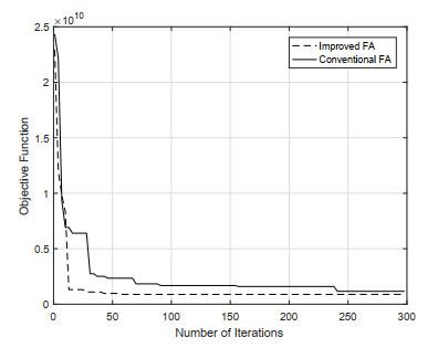
Number of Iterations	243	58
Objective Function g	1.1602 × 10⁹	8.8554 × 10⁸
Model's Coefficient of Determination R²	0.9989	0.9992

Figure 1 Curve graph of two algorithms' objective function value changes with iterations

Full size|PPT slide

L (t)

's curve equation is:

{\begin{array}{l} A = 1.3758 e^{0.0422 t}, \\ K = 15080 e^{0.1646 t}, \\ L = 68610 e^{0.0060 t}, \\ E = 99830 e^{0.06694 t}, \\ C = 18010 e^{0.1236 t}, \\ I = 33390 e^{0.0966 t}, \\ Y = 47710 e^{0.1220 t} . \end{array} 1 \leq t \leq 23 .

In this case, in the period from 1994 to 2016, the contribution rates of factors to economic growth are as follows:

Technological progress

A

's contribution rate is

\frac{Δ Y_{A}}{Δ Y} = 29.32 %;

factor

K

's contribution rate is

\frac{Δ Y_{K}}{Δ Y} = 36.52 %;

factor

L

's contribution rate is

\frac{Δ Y_{L}}{Δ Y} = 4.45 %;

factor

E

's contribution rate is

\frac{Δ Y_{E}}{Δ Y} = 12.91 %;

factor

C

's contribution rate is

\frac{Δ Y_{C}}{Δ Y} = 10.54 %;

factor

I

's contribution rate is

\frac{Δ Y_{I}}{Δ Y} = 6.26 % .

Calculation results show that Chinese economic growth depends mainly on capital input, next on technological progress and energy input, and then on consumption and import & export, and labor force makes less contribution. The result consists with the reality in China.

5 Conclusion

The paper proposes a new mixed production function model and uses an improved FA with the high precision and a fast convergence rate for the parameter estimation of model. With regard to the calculation of influencing factors' contribution rates to economic growth, traditional methods have big errors and are not applicable to complicated models, so the paper gives a scientific calculation method. The practical calculation proves that the method is reliable, accurate and highly exercisable. The idea and method given in the paper have important significance for the in-depth research on and wide application of production function model.

References

Publishing order | Descend order by publishing year | Descend order by cited within

1	Avvakumov S N, Kiselev Y N, Orlov M V, et al. Profit maximization problem for Cobb-Douglas and CES production functions. Computational Mathematics and Modeling, 2010, 21 (3): 336- 378. https://doi.org/10.1007/s10598-010-9075-5 Cited in this article [1]

2	Cheng M L. A new measure model of factor contribution ratio for economic growth. Mathematics in Economics, 2004, 21 (3): 235- 239. https://doi.org/10.3969/j.issn.1007-1660.2004.03.008

3	Cheng M L. China forecasting model of economic growth based on production function. Statistics and Decision, 2010, (20): 34- 36.

4	Kemfert C. Estimated substitution elasticities of a nested CES production function approach for Germany. Energy Economics, 1998, 20, 249- 264. https://doi.org/10.1016/S0140-9883(97)00014-5 Cited in this article [1]

5	Cheng M L. Correction and empirical analysis of the CES production function model. Journal of Engineering Mathematics, 2013, 30 (4): 535- 544. https://doi.org/10.3969/j.issn.1005-3085.2013.04.006 Cited in this article [1]

6	Cheng M L, Han Y. The measure model and analysis of contribution ratio of economic growth factor on Suzhou foreign capital manufacturing. Application of Statistics and Management, 2009, 28 (3): 381- 385.

7	Cheng M L, Han Y. A modified Cobb-Douglas production function model and its application. IMA Journal of Management Mathematics, 2014, 25 (3): 353- 365. https://doi.org/10.1093/imaman/dpt012

8	Hang B L, Wang W R, Ding L Q. An expand application to the CES production function. Quantitative & Technica Economics, 1997, (8): 52- 55.

9	Li Z N, Pang W Q. Econometrics. Beijing: Higher Education Press, 2010.

10	Cheng M L, Han Y. Application of a new superposition CES production function model. Journal of Systems Science and Information, 2017, 5 (5): 462- 472. https://doi.org/10.21078/JSSI-2017-462-11 Cited in this article [1]

11	Alrefaei M H, Diabat A H. A simulated annealing technique for multi-objective simulation optimization. Applied Mathematics and Computation, 2009, 215, 3029- 3035. https://doi.org/10.1016/j.amc.2009.09.051 Cited in this article [1]

12	Gaoa Y, Guana L, Wangb T. Optimal artificial fish swarm algorithm for the field calibration on marine navigation. Measurement, 2014, 50, 297- 304. https://doi.org/10.1016/j.measurement.2014.01.003

13	Neshat M, Sepidnam G, Sargolzaei M, et al. Artificial fish swarm algorithm: A survey of the state-of-the-art, hybridization, combinatorial and indicative applications. Artificial Intelligence Review, 2014, 42 (4): 965- 997. https://doi.org/10.1007/s10462-012-9342-2

14	Nie L M, Zhou Y Q. Using artificial fish-swarm algorithm for solving two-dimensional numerical integration. Computer Engineering and Applications, 2009, 45 (10): 34- 37.

15	Peng J S, Li X, Qin Z Q, et al. Robot global path planning based on improved artificial fish-swarm algorithm. Research Journal of Applied Sciences, Engineering and Technology, 2013, 5 (6): 2042- 2047.

16	Yang X M, Yuan J S, Yuan J Y, et al. A modified particle swarm optimizer with dynamic adaptation. Applied Mathematics and Computation, 2007, 189, 1205- 1213. https://doi.org/10.1016/j.amc.2006.12.045 Cited in this article [1]

17	Chen G Y, Ding X Q. Optimal economic dispatch with valve loading effect using self-adaptive firefly algorithm. Applied Intelligence, 2015, 42, 276- 288. https://doi.org/10.1007/s10489-014-0593-2 Cited in this article [1]

18	Gandomi A H, Yang X S, Talatahari S, et al. Firefly algorithm with chaos. Communications in Nonlinear Science and Numerical Simulation, 2013, 18, 89- 98. https://doi.org/10.1016/j.cnsns.2012.06.009

19	Mozaffari A, Azad N L. Coupling a chaotically encoded firefly algorithm with ranking to a physics-based mathematical model for robust optimisation of a gas turbine energy system. International Journal of Mathematical Modelling and Numerical Optimisation, 2014, 5, 295- 317.

20	Yu S H, Su S B, Lu Q P, et al. A novel wise step strategy for firefly algorithm. International Journal of Computer Mathematics, 2014, 91, 2507- 2513. Cited in this article [1]

21	Yan M, Wang W G. Estimating the contribution rate of education investment in the economic growth based on time-varying parameter. Statistics & Information Forum, 2009, 24 (7): 72- 78. Cited in this article [1]

22	Zhou S S, Hu D L. Research on contribution rate of science and technology progress to economy growth. China Soft Science, 2010, (2): 34- 39.

23	Cheng M L. A generalized constant elasticity of substitution production function model and its application. Journal of Systems Science and Information, 2016, 4 (3): 269- 279. https://syssci.cjoe.ac.cn/EN/10.21078/JSSI-2016-269-11 Cited in this article [1]

Funding

the National Natural Science Foundation of China(11401418)

PDF(144 KB)

153

Accesses

Citation

Detail

Sections

Recommended

Abstract
Key words
Cite this article
1 Introduction
2 Parameter Estimation of Mixed Production Function Model
2.1 Standard FA
2.2 Improved FA
2.3 Steps of Parameter Estimation Based on Improved FA
3 Calculation Method of Contribution Rate of Economic Growth Factors
4 Calculation of Contribution Rates of Chinese Economic Growth Factors
Table 1 Information of Chinese economic growth
Table 2 Comparison of results from different algorithms
Figure 1 Curve graph of two algorithms' objective function value changes with iterations
5 Conclusion
References
Funding

Received	Accepted	Published
2017-08-24	2017-12-07	2018-08-25
Issue Date
2018-08-25

Please choose a citation manager

Content to export

Abstract

Key words

Cite this article

1 Introduction

2 Parameter Estimation of Mixed Production Function Model

2.1 Standard FA

2.2 Improved FA

2.3 Steps of Parameter Estimation Based on Improved FA

3 Calculation Method of Contribution Rate of Economic Growth Factors

4 Calculation of Contribution Rates of Chinese Economic Growth Factors

Table 1 Information of Chinese economic growth

Table 2 Comparison of results from different algorithms

Figure 1 Curve graph of two algorithms' objective function value changes with iterations

5 Conclusion

{{custom_sec.title}}

{{custom_sec.title}}

References

{{custom_fnGroup.title_en}}

Footnotes

Funding

Share

模态框（Modal）标题

Please choose a citation manager

Content to export

Abstract

Key words

Cite this article

1 Introduction

2 Parameter Estimation of Mixed Production Function Model

2.1 Standard FA

2.2 Improved FA

2.3 Steps of Parameter Estimation Based on Improved FA

3 Calculation Method of Contribution Rate of Economic Growth Factors

4 Calculation of Contribution Rates of Chinese Economic Growth Factors

Table 1 Information of Chinese economic growth

Table 2 Comparison of results from different algorithms

Figure 1 Curve graph of two algorithms' objective function value changes with iterations

5 Conclusion

{{custom_sec.title}}

{{custom_sec.title}}

References

{{custom_fnGroup.title_en}}

Footnotes

Funding