Analysis of a Discrete-Time Geo/G/1 Queue in a Multi-Phase Service Environment with Disasters

Tao JIANG

doi:10.21078/JSSI-2018-349-17

PDF(190 KB)

Journal of Systems Science and Information ›› 2018, Vol. 6 ›› Issue (4) : 349-365. DOI: 10.21078/JSSI-2018-349-17

Analysis of a Discrete-Time Geo/G/1 Queue in a Multi-Phase Service Environment with Disasters

Author information +

History +

Abstract

This paper considers a discrete-time Geo/G/1 queue in a multi-phase service environment, where the system is subject to disastrous breakdowns, causing all present customers to leave the system simultaneously. At a failure epoch, the server abandons the service and the system undergoes a repair period. After the system is repaired, it jumps to operative phase i with probability q_i, i=1, 2 …, n. Using the supplementary variable technique, we obtain the distribution for the stationary queue length at the arbitrary epoch, which are then used for the computation of other performance measures. In addition, we derive the expected length of a cycle time, the generating function of the sojourn time of an arbitrary customer, and the generating function of the server's working time in a cycle. We also give the relationship between the discrete-time queueing system to its continuous-time counterpart. Finally, some examples and numerical results are presented.

Key words

discrete-time / Geo/G/1 queue / multi-phase service environment / disasters / supplementary variable technique

Cite this article

EndNote

Ris (Procite)

Bibtex

Download Citations

Tao JIANG. Analysis of a Discrete-Time Geo/G/1 Queue in a Multi-Phase Service Environment with Disasters. Journal of Systems Science and Information, 2018, 6(4): 349-365 https://doi.org/10.21078/JSSI-2018-349-17

1 Introduction

Queues with disasters have been intensively studied in the past by various researchers due to their great applications in complex modern communication systems, networks and manufacturing systems. The interested readers are referred to [1−10] and references therein. Since the discrete-time queue is more suitable for describing the telecommunication network, digital communication systems and other related areas, there is a growing interest in the analysis of the discrete-time queues with disasters. For example, Atencia and Moreno^[11] studied a Geo/Geo/1 queue with negative customers and disasters, and derived an explicit expression for the stationary distribution. Laterly, Yi, et al.^[12] analyzed the queue length of a Geo/G/1 queue with disasters and obtained the stationary queue length distribution. Moreover, using the results, the authors also analyzed a Geo/G/1 queue with multiple working vacations. Park, et al.^[13] extended the Geo/Geo/1 queue with negative customers and disasters to the Geo/G/1 queue, and provided the probability generating functions (PGFs) of the stationary queue length and sojourn time. In succession, the authors^[14] extended the Geo/Geo/1 queue with disasters to the GI/Geo/1 queue, in which the interarrival times of customers follow a general distribution. Furthermore, Lee, et al.^[15] discussed a discrete-time single server Geo/G/1 queue with disasters and general repair time. Lee and Yang^[16] studied an

N

-policy of a discrete-time Geo/G/1 queue with disasters in order to analyze the power saving scheme in wireless sensor networks under unreliable network connections.

The motivation for treating this type of queueing systems comes from several fields, especially in complex modern communication networks, transportation and manufacturing networks, etc. For example, in an unreliable multi-product manufacturing network, the service intensities to different production centers may vary depending on the type of jobs it is processing, environmental conditions and operator experience, and service process may be interrupted by some external factors. Also, the queueing model can be applied to a power saving scheme in wireless sensor networks (WSNs) under unreliable network connections where data packets may be lost by external attacks or shocks. Inspired by these applications, we aim to study a Geo/G/1 queue operating in a multi-phase service environment with disasters. More important, in this present paper, we derive the explicit PGF of the sojourn time of an arbitrary customer and the PGF of the server's working time in a cycle, which are the important performance measures in analyzing the queueing system. We also provide the cycle analysis and the relationship between the discrete-time system to its continuous-time counterpart.

The rest of the paper is organized as follows. In Section 2, we describe our queueing model. In Section 3, by using the supplementary variable technique, we define a Markov process and derive the PGF of the stationary queue size at an arbitrary epoch. Section 4 and Section 5 are devoted to giving the expected length of cycle time and the sojourn time distribution of an arbitrary customer. In Section 6, we give the relationship between the discrete-time system to its continuous-time counterpart. Some examples and numerical results are presented in Section 7. We conclude the paper in Section 8.

2 Model Description

In this paper, we consider a discrete-time Geo/G/1 queue operating in a multi-phase random environment with disasters. The queuing model is described in detail below:

1) Under operative phase

i, i = 1, 2, \dots, n

, customers arrive according to a Bernoulli arrival process with parameter

λ_{i}

, where

λ_{i}

is the probability that an arrival occurs in a slot. That is, in operative phase

i

, the interarrival times of customers

A_{i}

follow a geometric distribution. The probability mass function and its PGF are respectively denoted by

\begin{array}{rcl} P (A_{i} = k) = {\bar{λ}}_{i}^{k - 1} λ_{i}, k \geq 1, 0 < λ_{i} < 1, {\bar{λ}}_{i} = 1 - λ_{i}, \\ A_{i} (z) = \sum_{k = 1}^{\infty} P (A_{i} = k) z^{k} = \frac{λ_{i} z}{1 - {\bar{λ}}_{i} z} . \end{array}

2) Service times

S_{i}

are independent and identically distributed (iid) with a general (arbitrary) distribution with mean

E [S_{i}] = \frac{1}{μ_{i}}

. The probability mass function and its PGF are respectively denoted by

s_{i, k} = P (S_{i} = k), k \geq 1, S_{i} (z) = \sum_{k = 1}^{\infty} s_{i, k} z^{k} .

3) In operative phase

i

, the interarrival times of disasters

D_{i}

are geometrically distributed with parameter

η_{i}, i = 1, 2, \dots, n

. The probability mass function and its PGF are respectively denoted by

\begin{array}{rcl} P (D_{i} = k) = {\bar{η}}_{i}^{k - 1} η_{i}, k \geq 1, 0 < η_{i} < 1, {\bar{η}}_{i} = 1 - η_{i}, \\ D_{i} (z) = \sum_{k = 1}^{\infty} P (D_{i} = k) z^{k} = \frac{η_{i} z}{1 - {\bar{η}}_{i} z} . \end{array}

4) When the system is in operative phase

i, i = 1, 2, \dots, n

, it occasionally suffers a disastrous breakdown, forcing all customers to leave the system simultaneously. At a failure instant, the system moves to phase 0 (repair phase) and undergoes a repair process immediately with stopping service completely. Repair times follow a geometric distribution with parameter

η_{0}

. The probability mass function and its PGF are respectively denoted by

\begin{array}{rcl} P (T_{0} = k) = {\bar{η}}_{0}^{k - 1} η_{0}, k \geq 1, 0 < η_{0} < 1, {\bar{η}}_{0} = 1 - η_{0}, \\ T_{0} (z) = \sum_{k = 1}^{\infty} P (T_{0} = k) z^{k} = \frac{η_{0} z}{1 - {\bar{η}}_{0} z} . \end{array}

5) In phase 0, the parameter of the Bernoulli arrival process is

λ_{0}

, that is, the interarrival times of customers in repair period follow a geometric distribution. The probability mass function and its PGF are respectively denoted by

\begin{array}{rcl} P (A_{0} = k) = {\bar{λ}}_{0}^{k - 1} λ_{0}, k \geq 1, 0 < λ_{i} < 1, {\bar{λ}}_{0} = 1 - λ_{0}, \\ A_{0} (z) = \sum_{k = 1}^{\infty} P (A_{0} = k) z^{k} = \frac{λ_{0} z}{1 - {\bar{λ}}_{0} z} . \end{array}

We assume that the arriving customers enter the system in accordance with the first-come-first-served (FCFS) discipline. After the system is repaired, it moves from the repair phase to operative phase

i

with probability

q_{i}

, where

\sum_{i = 1}^{n} q_{i} = 1

. In this system, there is no direct jump among the operative phases. When a disaster occurs, the system must move to the repair phase, and then moves back to the operative phase

i

with probability

q_{i}

For the discrete-time queueing system in consideration, we consider the late arrival system (LAS) in which the time axis is divided into a sequence of intervals of equal length (i.e., slots) and the time axis is marked by

t = 0, 1, \dots

. According to the LAS model, a potential customer arrival occurs during the interval

(t^{-}, t)

, and a potential service completion takes place in

(t, t^{+})

, where

t^{+}

and

t^{-}

represent

lim_{Δ t \to 0} (t + | Δ t |)

and

lim_{Δ t \to 0} (t - | Δ t |)

, respectively. We also assume that a disaster arrival or its repair completion occurs at the instant

t

, that is, an arrival occurs at the epoch just before a slot boundary, a disaster arrival or a repair completion just at a slot boundary, and a service completion just after the slot boundary. We further assume that a disaster arrival and a repair completion don't occur simultaneously at the same slot boundary.

3 Stationary Queue Size Distribution

In this section, we use the supplementary variable technique to derive the stationary queue size at an arbitrary epoch. We note that as long as

η_{i} > 0, i = 0, 1, \dots, n

, that is, the existence of disasters, the system in consideration is stable. So we could analyze the system in steady state.

At an arbitrary time

t^{+}

, the system can be described by the process

{L (t^{+}), J (t^{+}), S^{+} (t^{+}), t = 0, 1, \dots},

where

L (t^{+})

is the number of customers in the system at time

t^{+}

J (t^{+})

denotes the phase in which the system operates at time

t^{+}

. If

L (t^{+}) \geq 1

J (t^{+}) = i

, then

S^{+} (t^{+}) = S_{i}^{+} (t^{+})

represents the remaining service time of the customer currently being served during operative phase

i, i = 1, 2, \dots, n

. Hence,

{L (t^{+}), J (t^{+}), S^{+} (t^{+}), t = 0, 1, \dots}

is a discrete-time Markov chain in which the supplementary variables are

S^{+} (t^{+}) = S_{i}^{+} (t^{+}), i = 1, 2, \dots, n

with the state space

Ω = {(m, 0), m \geq 0} \cup {(0, i), (m, i, k), m \geq 1, k \geq 1, i = 1, 2, \dots, n} .

We first define the following limiting probabilities:

\begin{array}{rcl} P_{m, 0} = lim_{t \to \infty} P {L (t^{+}) = m, J (t^{+}) = 0}, m \geq 0, \\ P_{0, i} = lim_{t \to \infty} P {L (t^{+}) = 0, J (t^{+}) = i, i = 1, 2, \dots, n}, \\ P_{m, i} (k) = lim_{t \to \infty} P {L (t^{+}) = m, J (t^{+}) = i, S_{i}^{+} (t^{+}) = k, m \geq 1, i = 1, 2, \dots, n, k \geq 1} . \end{array}

Using these limiting probabilities and the supplementary variable technique, we can easily establish the following balance equations:

\begin{array}{rcl} P_{0, 0} = {\bar{λ}}_{0} {\bar{η}}_{0} P_{0, 0} + \sum_{i = 1}^{n} η_{i} [\sum_{m = 1}^{\infty} \sum_{k = 1}^{\infty} P_{m, i} (k) + P_{0, i}], \end{array}

(1)

\begin{array}{rcl} P_{m, 0} = {\bar{λ}}_{0} {\bar{η}}_{0} P_{m, 0} + λ_{0} {\bar{η}}_{0} P_{m - 1, 0}, m \geq 1, \end{array}

(2)

\begin{array}{rcl} P_{0, i} = {\bar{λ}}_{i} {\bar{η}}_{i} P_{0, i} + {\bar{λ}}_{i} {\bar{η}}_{i} P_{1, i} (1) + q_{i} {\bar{λ}}_{0} η_{0} P_{0, 0}, i = 1, 2, \dots, n, \end{array}

(3)

\begin{array}{rcl} P_{1, i} (k) = {\bar{η}}_{i} [λ_{i} s_{i, k} P_{0, i} + {\bar{λ}}_{i} P_{1, i} (k + 1) + λ_{i} s_{i, k} P_{1, i} (1) + {\bar{λ}}_{i} s_{i, k} P_{2, i} (1)] \\ + η_{0} q_{i} s_{i, k} ({\bar{λ}}_{0} P_{1, 0} + λ_{0} P_{0, 0}), i = 1, 2, \dots, n, \end{array}

(4)

\begin{array}{rcl} P_{m, i} (k) = {\bar{η}}_{i} [λ_{i} P_{m - 1, i} (k + 1) + {\bar{λ}}_{i} P_{m, i} (k + 1) + λ_{i} s_{i, k} P_{m, i} (1) + {\bar{λ}}_{i} s_{i, k} P_{m + 1, i} (1)] \\ + η_{0} q_{i} s_{i, k} ({\bar{λ}}_{0} P_{m, 0} + λ_{0} P_{m - 1, 0}), m \geq 2, i = 1, 2, \dots, n, \end{array}

(5)

where

{\bar{λ}}_{0} = 1 - λ_{0}, {\bar{η}}_{0} = 1 - η_{0}, {\bar{λ}}_{i} = 1 - λ_{i}, {\bar{η}}_{i} = 1 - η_{i}, i = 1, 2, \dots, n

In order to obtain the solutions of the set of equations, we further define the following generating functions:

\begin{array}{rcl} P_{0} (z) = \sum_{m = 0}^{\infty} P_{m, 0} z^{m}, | z | < 1, \\ P_{i} (k, z) = \sum_{m = 1}^{\infty} P_{m, i} (k) z^{m}, i = 1, 2, \dots, n, k \geq 1, | z | < 1, \\ P_{i}^{*} (x, z) = \sum_{k = 1}^{\infty} P_{i} (k, z) x^{k} = \sum_{k = 1}^{\infty} \sum_{m = 1}^{\infty} P_{m, i} (k) z^{m} x^{k}, i = 1, 2, \dots, n, | x | < 1, | z | < 1. \end{array}

First, from (2), we have

P_{m, 0} = \frac{λ_{0} {\bar{η}}_{0}}{1 - {\bar{λ}}_{0} {\bar{η}}_{0}} P_{m - 1, 0} = {(\frac{λ_{0} {\bar{η}}_{0}}{1 - {\bar{λ}}_{0} {\bar{η}}_{0}})}^{m} P_{0, 0} .

(6)

Then,

P_{0} (z)

can be obtained by

P_{0} (z) = \sum_{m = 0}^{\infty} P_{m, 0} z^{m} = \sum_{m = 0}^{\infty} {(\frac{λ_{0} {\bar{η}}_{0}}{1 - {\bar{λ}}_{0} {\bar{η}}_{0}})}^{m} z^{m} P_{0, 0} = \frac{1 - {\bar{λ}}_{0} {\bar{η}}_{0}}{1 - {\bar{λ}}_{0} {\bar{η}}_{0} - λ_{0} {\bar{η}}_{0} z} P_{0, 0} .

(7)

Multiplying (4) and (5) by

z

and

z^{m}

, summing over

m

, and then simplifying the result with (3), we have

\begin{array}{rcl} P_{i} (k, z) & = & α_{i} (z) P_{i} (k + 1, z) + s_{i, k} [z^{- 1} α_{i} (z) P_{i} (1, z) + (α_{i} (z) - 1) P_{0, i} \\ + q_{i} η_{0} P_{0} (z) ({\bar{λ}}_{0} + z λ_{0})], i = 1, 2, \dots, n, k \geq 1, \end{array}

(8)

where

α_{i} (z) = z λ_{i} {\bar{η}}_{i} + {\bar{λ}}_{i} {\bar{η}}_{i}, i = 1, 2, \dots, n

Multiplying (8) by

x^{k}

, and then summing over

k

, we obtain

\begin{array}{rcl} (1 - α_{i} (z) x^{- 1}) P_{i}^{*} (x, z) & = & z^{- 1} α_{i} (z) P_{i} (1, z) [S_{i} (x) - z] \\ + S_{i} (x) [(α_{i} (z) - 1) P_{0, i} + q_{i} η_{0} P_{0} (z) (\bar{λ_{0}} + z λ_{0})] . \end{array}

(9)

Choosing

x = α_{i} (z)

and substituting it into (9), we have

P_{i} (1, z) = \frac{z S_{i} (α_{i} (z)) [(α_{i} (z) - 1) P_{0, i} + q_{i} η_{0} P_{0} (z) ({\bar{λ}}_{0} + z λ_{0})]}{α_{i} (z) [z - S_{i} (α_{i} (z))]} .

(10)

Lemma 1

z = S_{i} (α_{i} (z))

has a unique root in

| z | < 1

, where

α_{i} (z) = z λ_{i} {\bar{η}}_{i} + {\bar{λ}}_{i} {\bar{η}}_{i}, i = 1, 2, \dots, n

Proof The method for the proof of Lemma 1 is similar to Appendix A of [15], and we do not explain it here any more.

By Lemma 1,

P_{0, i}

can be obtained by

P_{0, i} = \frac{q_{i} η_{0} P_{0} (γ_{i}) ({\bar{λ}}_{0} + γ_{i} λ_{0})}{(1 - α_{i} (γ_{i}))},

(11)

where

γ_{i}

is the unique root of

z = S_{i} (α_{i} (z))

| z | < 1

Substituting (10) into (9), we have

P_{i}^{*} (x, z) = \frac{z x [S_{i} (x) - S_{i} (α_{i} (z))] [(α_{i} (z) - 1) P_{0, i} + q_{i} η_{0} P_{0} (z) ({\bar{λ}}_{0} + z λ_{0})]}{(x - α_{i} (z)) [z - S_{i} (α_{i} (z))]} .

(12)

By using the normalizing condition

P_{0} (1) + \sum_{i = 1}^{n} [P_{i}^{*} (1, 1) + P_{0, i}] = 1,

(13)

we have

P_{0, 0} = \frac{1}{(1 - {\bar{λ}}_{0} {\bar{η}}_{0}) β},

where

β = \frac{1}{η_{0}} + \sum_{i = 1}^{n} \frac{q_{i}}{η_{i}}

, and it represents the expected length of time between two consecutive epochs at which a repair phase commences.

Define

P (z)

as the PGF of the queue length, then,

P (z)

can be obtained by

P (z) = P_{0} (z) + \sum_{i = 1}^{n} [P_{i}^{*} (1, z) + P_{0, i}],

where

P_{i}^{*} (1, z) = \frac{z [1 - S_{i} (α_{i} (z))] [(α_{i} (z) - 1) P_{0, i} + q_{i} η_{0} P_{0} (z) ({\bar{λ}}_{0} + z λ_{0})]}{(1 - α_{i} (z)) [z - S_{i} (α_{i} (z))]} .

4 Performance Measures

In this section, based on the obtained results, we give some performance measures. First, let

L

denote the stationary random variable for the number of customers in the system.

The expected number of customers in the system is

\begin{array}{rcl} E [L] & = & {\frac{d P (z)}{d z} |}_{z = 1} \\ = & \frac{λ_{0} {\bar{η}}_{0}}{η_{0}^{2} β} + \sum_{i = 1}^{n} \frac{1}{η_{i}} [(λ_{i} {\bar{η}}_{i} - η_{i}) P_{0, i} + \frac{q_{i} η_{0} (1 + λ_{0}) + q_{i} λ_{0} {\bar{η}}_{0}}{η_{0} β}] \\ - \sum_{i = 1}^{n} \frac{1}{η_{i}} \frac{q_{i} - β η_{i} P_{0, i}}{β [1 - S_{i} ({\bar{η}}_{i})]} - \sum_{i = 1}^{n} \frac{(β η_{i} P_{0, i} - q_{i}) λ_{i} {\bar{η}}_{i}}{β η_{i}^{2}} . \end{array}

(14)

The system is empty with probability

\begin{array}{rcl} P_{0} & = & P_{0, 0} + \sum_{i = 1}^{n} P_{0, i} \\ = & [\sum_{i = 1}^{n} \frac{q_{i} η_{0} ({\bar{λ}}_{0} + γ_{i} λ_{0})}{[1 - α_{i} (γ_{i})] (1 - {\bar{λ}}_{0} {\bar{η}}_{0} - λ_{0} {\bar{η}}_{0} γ_{i})} + \frac{1}{1 - {\bar{λ}}_{0} {\bar{η}}_{0}}] \frac{1}{β} . \end{array}

(15)

The system is in phase

i

with probability

P_{i} = P_{i}^{*} (1, 1) + P_{0, i} = \frac{q_{i} η_{0} P_{0} (1)}{η_{i}} = \frac{q_{i}}{β η_{i}}, i = 1, 2, \dots, n .

(16)

Notice that the stochastic process in consideration can be reduced to a modified alternating renewal process. Since there are

n + 1

phases in this queueing model, we can define

n + 1

types of cycle and give the cycle analysis. First, let

C_{i}

denote the length of time between two consecutive epochs at which phase

i

commences,

i = 0, 1, 2, \dots, n

, i.e., the length of type-

i

cycle. Obviously,

E [C_{0}] = β

, that is the expected length of type-

0

cycle equals to

β

. Next, we aim to derive the expected length of type-

i

cycle for

i = 1, 2, \dots, n

It is not difficult to see that the probability that the system goes through the repair phase

k

times between two successive visits at phase

i

(1 - q_{i})^{k - 1} q_{i}, k \geq 1

, and the expected length of time between two consecutive epochs at which phase

i

commences in this case is

(\frac{1}{η_{i}} + \frac{1}{η_{0}}) + (k - 1) (\frac{1}{η_{0}} + \sum_{j = 1, j \neq i}^{n} \frac{q_{j}}{η_{j} (1 - q_{i})})

. Therefore,

E [C_{i}]

can be obtained by

\begin{array}{rcl} E [C_{i}] & = & \sum_{k = 1}^{\infty} {(1 - q_{i})}^{k - 1} q_{i} [(\frac{1}{η_{i}} + \frac{1}{η_{0}}) + (k - 1) (\frac{1}{η_{0}} + \sum_{j = 1, j \neq i}^{n} \frac{q_{j}}{η_{j} (1 - q_{i})})] \\ = & (\frac{1}{η_{i}} + \frac{1}{η_{0}}) + \sum_{k = 1}^{\infty} (k - 1) {(1 - q_{i})}^{k - 1} q_{i} [\frac{1}{η_{0}} + (β - \frac{1}{η_{0}} - \frac{q_{i}}{η_{i}}) \frac{1}{1 - q_{i}}] \\ = & (\frac{1}{η_{i}} + \frac{1}{η_{0}}) + \frac{1 - q_{i}}{q_{i}} [\frac{- q_{i}}{η_{0} (1 - q_{i})} + (β - \frac{q_{i}}{η_{i}}) \frac{1}{1 - q_{i}}] \\ = & \frac{1}{η_{i}} + \frac{1}{q_{i}} (β - \frac{q_{i}}{η_{i}}) \\ = & \frac{β}{q_{i}}, i = 1, 2, \dots, n . \end{array}

(17)

Next, we will derive the PGF of the stationary sojourn time of an arbitrary customer by considering a tagged customer, which is defined to be the overall time since the arrival till the departure from the system, by either the service completion or occurrence of a disaster. Let

W

and

W (z)

respectively denote the stationary sojourn time of an arbitrary customer and its PGF. For this discrete-time queueing system, a tagged customer's arriving which occurs in

(t^{-}, t)

may belong to one of the following four possible cases:

Case 1: the tagged customer arrives in the state

(0, i), i = 1, 2, \dots, n

;

Case 2: the tagged customer arrives in the state

(m, i, k), m \geq 1, k \geq 0, i = 1, 2, \dots, n

;

Case 3: the tagged customer arrives in the state

(0, 0)

;

Case 4: the tagged customer arrives in the state

(m, 0), m \geq 1

For the further calculation, we first give a lemma below.

Lemma 2 Let $X, Y, Z$ be the discrete random variables with positive integer value, and $Z = min (X, Y)$ , where $X$ follows a general $($ arbitrary $)$ distribution with mean $\frac{1}{μ}$ . The probability mass function and its PGF are respectively denoted by $P (X = k)$ and $X (z)$ , $Y$ follows an geometric distribution with parameter $η$ , and $X$ and $Y$ are assumed to be independent. Define $G (z)$ as the PGF of random variable $Z$ . Then

G (z) = \frac{η z + (1 - z) X (\bar{η} z)}{1 - \bar{η} z} .

Proof First, we have the distribution law of

Z

\begin{array}{rcl} P {Z = min (X, Y) = k} & = & P {Y = k, X \geq k} + P {X = k, Y \geq k + 1} \\ = & η {\bar{η}}^{k - 1} P {X \geq k} + {\bar{η}}^{k} P {X = k} . \end{array}

(18)

Then, the PGF of

Z

can be expressed as

\begin{array}{rcl} G (z) & = & \sum_{k = 1}^{\infty} η {\bar{η}}^{k - 1} P {X \geq k} z^{k} + X (\bar{η} z) \\ = & \sum_{k = 1}^{\infty} η {\bar{η}}^{k - 1} \sum_{i = k}^{\infty} P {X = i} z^{k} + X (\bar{η} z) \\ = & η z \sum_{k = 1}^{\infty} {(\bar{η} z)}^{k - 1} \sum_{i = k}^{\infty} P {X = i} + X (\bar{η} z) \\ = & η z \sum_{i = 1}^{\infty} \sum_{k = 1}^{i} P {X = i} {(\bar{η} z)}^{k - 1} + X (\bar{η} z) \\ = & \frac{η z [1 - X (\bar{η} z)]}{1 - \bar{η} z} + X (\bar{η} z) = \frac{η z + (1 - z) X (\bar{η} z)}{1 - \bar{η} z} . \end{array}

(19)

So, we can obtain the conclusion.

Define

D_{i}

as the duration of time that the system resides in operative phase

i

T_{m, i}

as the total service time of

m

customers in operative phase

i

. In Case 1, upon the tagged customer arrives, he immediately receives service and leaves the system by either the service completion or the occurrence of a disaster. Let

W_{0, i}

denote the sojourn time of the tagged customer who arrives in Case 1, and define

W_{0, i} (z) = P (Case 1) E [z^{W_{0, i}} | Case 1] .

At a tagged customer arriving epoch, if the occurrence of diaster does not happen simultaneously at the slot boundary, then

W_{0, i}

has the relation:

W_{0, i} = min (S_{i}, D_{i})

, otherwise the sojourn time of this tagged customer is zero. So we have

\begin{array}{rcl} W_{0, i} (z) & = & P (Case 1) E [z^{W_{0, i}} | Case 1] \\ = & lim_{t \to \infty} P {L (t^{-}) = 0, J (t^{-}) = i} (η_{i} E [z^{0}] + {\bar{η}}_{i} E [z^{min (S_{i}, D_{i})}]) \\ = & lim_{t \to \infty} P {L ((t - 1)^{+}) = 0, J ((t - 1)^{+}) = i} (η_{i} E [z^{0}] + {\bar{η}}_{i} E [z^{min (S_{i}, D_{i})}]) \\ = & P_{0, i} (η_{i} E [z^{0}] + {\bar{η}}_{i} E [z^{min (S_{i}, D_{i})}]) \\ = & P_{0, i} (η_{i} + \bar{η_{i}} \frac{η_{i} z + (1 - z) S_{i} ({\bar{η}}_{i} z)}{1 - {\bar{η}}_{i} z}) . \end{array}

(20)

In Case 2, let

W_{m, i, k}

denote the sojourn time of the tagged customer who arrives in this case. Define

W_{m, i, k} (z) = P (Case2) E [z^{W_{m, i, k}} | Case2] .

Then, we have

\begin{array}{rcl} W_{m, i, k} (z) & = & P (Case2) E [z^{W_{m, i, k}} | Case2] \\ = & lim_{t \to \infty} P {L (t^{-}) = m, J (t^{-}) = i, S_{i}^{+} (t^{-}) = k} \\ \times {η_{i} E [z^{0}] + {\bar{η}}_{i} E [z^{min (k + T_{m, i}, D_{i})}]} \\ = & lim_{t \to \infty} P {L ({(t - 1)}^{+}) = m, J ({(t - 1)}^{+}) = i, S_{i}^{+} ({(t - 1)}^{+}) = k + 1} \\ \times {η_{i} + {\bar{η}}_{i} {P {D_{i} > k} z^{k} E [z^{min (T_{m, i}, D_{i})}] + \sum_{h = 1}^{k} P {D_{i} = h} z^{h}}} \\ = & P_{m, i} (k + 1) \\ \times {η_{i} + {\bar{η}}_{i} {P {D_{i} > k} z^{k} E [z^{min (T_{m, i}, D_{i})}] + \sum_{h = 1}^{k} P {D_{i} = h} z^{h}}} \\ = & P_{m, i} (k + 1) \\ \times {η_{i} + {\bar{η}}_{i} {{({\bar{η}}_{i} z)}^{k} \frac{η_{i} z + (1 - z) {[S_{i} ({\bar{η}}_{i} z)]}^{m})}{1 - {\bar{η}}_{i} z} + \frac{η_{i} z (1 - {({\bar{η}}_{i} z)}^{k})}{1 - {\bar{η}}_{i} z}}} \\ = & P_{m, i} (k + 1) \times {η_{i} + {\bar{η}}_{i} {\frac{{({\bar{η}}_{i} z)}^{k} (1 - z) {[S_{i} ({\bar{η}}_{i} z)]}^{m} + {\bar{η}}_{i} z}{1 - {\bar{η}}_{i} z}}} . \end{array}

(21)

Define

W_{i} (z) = \sum_{m = 1}^{\infty} \sum_{k = 0}^{\infty} W_{m, i, k} (z),

then,

\begin{array}{rcl} W_{i} (z) & = & \sum_{m = 1}^{\infty} \sum_{k = 0}^{\infty} W_{m, i, k} (z) \\ = & η_{i} P_{i}^{*} (1, 1) + \frac{(1 - z)}{1 - {\bar{η}}_{i} z} \frac{P_{i}^{*} (S_{i} ({\bar{η}}_{i} z), {\bar{η}}_{i} z)}{z} + \frac{η_{i} {\bar{η}}_{i} z}{1 - \bar{η_{i}} z} P_{i}^{*} (1, 1) \\ = & \frac{(1 - z)}{1 - {\bar{η}}_{i} z} \frac{P_{i}^{*} (S_{i} ({\bar{η}}_{i} z), {\bar{η}}_{i} z)}{z} + \frac{η_{i}}{1 - {\bar{η}}_{i} z} P_{i}^{*} (1, 1) . \end{array}

(22)

In Case 3, let

W_{0, 0}

denote the sojourn time in this case. Define

W_{0, 0} (z) = P (Case3) E [z^{W_{0, 0}} | Case 3],

then, we obtain

\begin{array}{rcl} W_{0, 0} (z) & = & P (Case3) E [z^{W_{0, 0}} | Case3] \\ = & lim_{t \to \infty} P {L (t^{-}) = 0, J (t^{-}) = 0} E [z^{W_{0, 0}} | Case3] \\ = & lim_{t \to \infty} P {L ((t - 1)^{+}) = 0, J ((t - 1)^{+}) = 0} E [z^{W_{0, 0}} | Case3] \\ = & P_{0, 0} (η_{0} E [z^{0}] \sum_{i = 1}^{n} q_{i} E [z^{min (S_{i}, D_{i})}] + {\bar{η}}_{0} \sum_{i = 1}^{n} q_{i} E [z^{T_{0} + min (S_{i}, D_{i})}]) \\ = & \frac{1}{(1 - {\bar{λ}}_{0} {\bar{η}}_{0}) β} [η_{0} + {\bar{η}}_{0} \frac{η_{0} z}{1 - {\bar{η}}_{0} z}] \sum_{i = 1}^{n} q_{i} \frac{η_{i} z + (1 - z) S_{i} ({\bar{η}}_{i} z)}{1 - {\bar{η}}_{i} z} . \end{array}

(23)

In Case 4, let

W_{m, 0}

denote the sojourn time in this case. Define

W_{m, 0} (z) = P (Case4) E [z^{W_{m, 0}} | Case4],

then, we have

\begin{array}{rcl} W_{m, 0} (z) & = & P (Case4) E [z^{W_{m, 0}} | Case4] \\ = & lim_{t \to \infty} P {L (t^{-}) = m, J (t^{-}) = 0} E [z^{W_{m, 0}} | C a s e 4] \end{array}

(24)

\begin{array}{rcl} [2 e x] & = & lim_{t \to \infty} P {L ((t - 1)^{+}) = m, J ((t - 1)^{+}) = 0} E [z^{W_{m, 0}} | C a s e 4] \\ = & P_{m, 0} E [z^{W_{m, 0}}] = P_{m, 0} [η_{0} + {\bar{η}}_{0} T_{0} (z)] \sum_{i = 1}^{n} q_{i} E [z^{min (T_{m + 1, i}, D_{i})}] \\ = & P_{m, 0} [η_{0} + {\bar{η}}_{0} \frac{η_{0} z}{1 - {\bar{η}}_{0} z}] \sum_{i = 1}^{n} q_{i} \frac{η_{i} z + (1 - z) {[S_{i} ({\bar{η}}_{i} z)]}^{m + 1}}{1 - {\bar{η}}_{i} z} . \end{array}

(25)

Finally, we obtain the PGF of the stationary sojourn time of an arbitrary customer

W (z) = \sum_{i = 1}^{n} W_{0, i} (z) + \sum_{i = 1}^{n} W_{i} (z) + W_{0, 0} (z) + \sum_{m = 1}^{\infty} W_{m, 0} (z) .

5 The Length of Working Time in a Cycle

In this section, we give the PGF of the server's working time in type-0 cycle. To avoid confusion, the working time is a period that the server is in working state in type-0 cycle. In order to derive the results, we first consider two types of cases:

Case 1: No arrivals during phase 0 (repair period);

Case 2:

k, k \geq 1

arrivals during phase 0 (repair period).

Next, we define

H_{i, 0}

as the length of working time in operative phase

i

under case 1,

H_{i, k}, k \geq 1

as the length of working time in operative phase

i

under case 2,

B_{i, k}

as the length of busy period caused by

k, k \geq 1

, customers in operative phase

i, i = 1, 2, \dots, n

In case 1, we further consider two cases: one is that no arrivals in operative phase

i

, and the other one is that customer arrivals occurring during phase

i, i = 1, 2, \dots, n

. Then, we have

\begin{array}{rcl} H_{i, 0} = {\begin{cases} 0, & A_{i} \geq D_{i}, \\ T, & A_{i} < D_{i}, \end{cases} T = {\begin{cases} T_{1}, & B_{i, 1} \geq D_{i}, \\ T_{2} + H_{i, 0}, & B_{i, 1} < D_{i}, \end{cases} \\ T_{1} = (D_{i} | B_{i, 1} \geq D_{i}), T_{2} = (B_{i, 1} | B_{i, 1} < D_{i}) . \end{array}

So, the PGF of

T_{1}

and

T_{2}

can be obtained as follows:

\begin{array}{rcl} T_{1} (z) & = & E [z^{D_{i}} | B_{i, 1} \geq D_{i}] \\ = & \frac{1}{P (B_{i, 1} \geq D_{i})} \sum_{m = 1}^{\infty} z^{m} P (D_{i} = m, B_{i, 1} \geq D_{i}) \\ = & \frac{1}{P (B_{i, 1} \geq D_{i})} \sum_{m = 1}^{\infty} z^{m} P (B_{i, 1} \geq D_{i} | D_{i} = m) P (D_{i} = m) \\ = & \frac{1}{P (B_{i, 1} \geq D_{i})} \sum_{m = 1}^{\infty} \sum_{k = m}^{\infty} z^{m} P (B_{i, 1} = k) P (D_{i} = m) \\ = & \frac{1}{P (B_{i, 1} \geq D_{i})} \sum_{k = 1}^{\infty} \sum_{m = 1}^{k} z^{m} {\bar{η}}_{i}^{m - 1} η_{i} P (B_{i, 1} = k) \\ = & \frac{η_{i} z}{1 - {\bar{η}}_{i} z} \frac{1 - B_{i, 1} ({\bar{η}}_{i} z)}{P (B_{i, 1} \geq D_{i})}, \end{array}

(26)

\begin{array}{rcl} T_{2} (z) & = & E [z^{B_{i, 1}} | B_{i, 1} < D_{i}] \\ = & \frac{1}{P (B_{i, 1} < D_{i})} \sum_{m = 1}^{\infty} \sum_{k = m + 1}^{\infty} z^{m} P (D_{i} = k) P (B_{i, 1} = m) \\ = & \frac{1}{P (B_{i, 1} < D_{i})} \sum_{m = 1}^{\infty} \sum_{k = m + 1}^{\infty} z^{m} {\bar{η}}_{i}^{k - 1} η_{i} P (B_{i, 1} = m) \\ = & \frac{B_{i, 1} ({\bar{η}}_{i} z)}{P (B_{i, 1} < D_{i})} . \end{array}

(27)

Substituting (26) and (27) into

T (z) = P (B_{i, 1} \geq D_{i}) T_{1} (z) + P (B_{i, 1} < D_{i}) T_{2} (z) H_{i, 0} (z),

we have

T (z) = \frac{η_{i} z}{1 - {\bar{η}}_{i} z} [1 - B_{i, 1} ({\bar{η}}_{i} z)] + B_{i, 1} ({\bar{η}}_{i} z) H_{i, 0} (z),

and

\begin{array}{rcl} H_{i, 0} (z) & = & P (A_{i} \geq D_{i}) E [z^{0}] + P (A_{i} < D_{i}) T (z) \\ = & \frac{η_{i}}{1 - {\bar{λ}}_{i} {\bar{η}}_{i}} + \frac{λ_{i} {\bar{η}}_{i}}{1 - {\bar{λ}}_{i} {\bar{η}}_{i}} [\frac{η_{i} z}{1 - {\bar{η}}_{i} z} [1 - B_{i, 1} ({\bar{η}}_{i} z)] + B_{i, 1} ({\bar{η}}_{i} z) H_{i, 0} (z)] . \end{array}

(28)

Simplifying (28), we have

H_{i, 0} (z) = \frac{η_{i} (1 - {\bar{η}}_{i} z) + λ_{i} {\bar{η}}_{i} η_{i} z [1 - B_{i, 1} ({\bar{η}}_{i} z)]}{[(1 - {\bar{λ}}_{i} {\bar{η}}_{i}) - λ_{i} {\bar{η}}_{i} B_{i, 1} ({\bar{η}}_{i} z)] (1 - {\bar{η}}_{i} z)},

where

B_{i, 1} ({\bar{η}}_{i} z)

satisfies

B_{i, 1} ({\bar{η}}_{i} z) = S_{i} [λ_{i} {\bar{η}}_{i} z B_{i, 1} ({\bar{η}}_{i} z) + {\bar{λ}}_{i} {\bar{η}}_{i} z]

Similarly to case 1, for case 2,

H_{i, k}

can be obtained by

H_{i, k} = {\begin{cases} Y_{1}, & B_{i, k} \geq D_{i}, \\ Y_{2} + H_{i, 0}, & B_{i, k} < D_{i}, \end{cases}

where

Y_{1} = (D_{i} | B_{i, k} \geq D_{i})

and

Y_{2} = (B_{i, k} | B_{i, k} < D_{i})

. And the PGF of

Y_{1}

and

Y_{2}

can be obtained as follows:

\begin{array}{rcl} Y_{1} (z) & = & \frac{η_{i} z}{1 - {\bar{η}}_{i} z} \frac{1 - B_{i, k} ({\bar{η}}_{i} z)}{P (B_{i, k} \geq D_{i})}, \\ Y_{2} (z) & = & \frac{B_{i, k} ({\bar{η}}_{i} z)}{P (B_{i, k} < D_{i})} . \end{array}

Substituting

Y_{1} (z)

and

Y_{2} (z)

into

H_{i, k} (z) = P (B_{i, k} \geq D_{i}) Y_{1} (z) + P (B_{i, k} < D_{i}) Y_{2} (z) H_{i, 0} (z)

, we have

H_{i, k} (z) = \frac{η_{i} z}{1 - {\bar{η}}_{i} z} [1 - B_{i, k} ({\bar{η}}_{i} z)] + B_{i, k} ({\bar{η}}_{i} z) Y_{2} (z) H_{i, 0} (z),

where

B_{i, k} ({\bar{η}}_{i} z) = [B_{i, 1} ({\bar{η}}_{i} z)]^{k}, k \geq 1

, and

B_{i, 1} ({\bar{η}}_{i} z)

satisfies

B_{i, 1} ({\bar{η}}_{i} z) = S_{i} [λ_{i} {\bar{η}}_{i} z B_{i, 1} ({\bar{η}}_{i} z) + {\bar{λ}}_{i} {\bar{η}}_{i} z]

Finally, we define

H

and

H (z)

as the length of working time in a type-0 cycle and its PGF,

a_{k}

as the probability that there are

k

arrivals during phase 0, and

a_{0}

as the probability that no arrivals during phase 0. Then, it is easy to derive that

\begin{array}{rcl} a_{0} & = & \sum_{r = 1}^{\infty} P (T_{0} = r) {\bar{λ}}_{0}^{r} = \frac{{\bar{λ}}_{0} η_{0}}{1 - {\bar{λ}}_{0} {\bar{η}}_{0}}, \\ a_{k} & = & \sum_{r = k}^{\infty} P (T_{0} = r) C_{r}^{k} {λ_{i}}^{k} {\bar{λ}}_{i}^{r - k}, k \geq 1 . \end{array}

Finally,

H (z)

can be obtained by

H (z) = \sum_{i = 1}^{n} q_{i} [a_{0} H_{i, 0} (z) + \sum_{k = 1}^{\infty} a_{k} H_{i, k} (z)] .

6 Relation to the Continuous-Time System

In this section, if we assume that the length of a slot is equal to a constant value

Δ

, not a time unit, we can use the similar method by referring to [17, 18] to analyze the relationship between the discrete-time system to its continuous-time counterpart by taking the limit

Δ \to 0

, that is, the continuous-time queueing system can be approximated by its corresponding discrete-time system.

We consider the continuous-time M/G/1 queue in multi-phase service environment with disasters. Under operative environment

i, i = 1, 2, \dots, n

, the Poisson arrival rate is

{\tilde{λ}}_{i}

, and the service times follow a general (arbitrary) distribution with mean

\frac{1}{{\tilde{μ}}_{i}}

. The distribution function and its Laplace Stieltjes transform (LST) respectively denoted by

B_{i} (x)

and

B_{i}^{*} (s)

. The duration of time that the system resides in phase

i

follows an exponential distribution with parameter

{\tilde{η}}_{i}, i = 0, 1, \dots, n

. If we assume that time is slotted into intervals of equal length

Δ

, we can approximate the continuous-time system by a discrete-time system for which

\begin{array}{rcl} λ_{i} = {\tilde{λ}}_{i} Δ, η_{i} = {\tilde{η}}_{i} Δ, i = 0, 1, \dots, n, \\ s_{i, k} = \int_{(k - 1) Δ}^{k Δ} d B_{i} (x), i = 1, 2, \dots, n, k \geq 1, \end{array}

where

Δ

is sufficiently small so that

λ_{i}

and

η_{i}

are probabilities.

Next, we can show that

lim_{Δ \to 0} P (z)

is the PGF of the number of customers in the continuous-time counterpart. First, we have

\begin{array}{rcl} lim_{Δ \to 0} P_{0} (z) & = & lim_{Δ \to 0} \frac{1}{(1 - {\bar{λ}}_{0} {\bar{η}}_{0} - λ_{0} {\bar{η}}_{0} z) β} \\ = & lim_{Δ \to 0} \frac{1}{[1 - (1 - {\tilde{λ}}_{0} Δ) (1 - {\tilde{η}}_{0} Δ) - {\tilde{λ}}_{0} Δ (1 - {\tilde{η}}_{0} Δ) z] (\frac{1}{{\tilde{η}}_{0} Δ} + \sum_{i = 1}^{n} \frac{q_{i}}{{\tilde{η}}_{i} Δ})} \\ = & \frac{1}{({\tilde{λ}}_{0} + {\tilde{η}}_{0} - {\tilde{λ}}_{0} z) (\frac{1}{{\tilde{η}}_{0}} + \sum_{i = 1}^{n} \frac{q_{i}}{{\tilde{η}}_{i}})} = {\tilde{P}}_{0} (z) . \end{array}

(29)

Second, using the same approach in [17, 18], we have

\begin{array}{rcl} lim_{Δ \to 0} S_{i} [{\bar{η}}_{i} ({\bar{λ}}_{i} + λ_{i} z)] \\ = & lim_{Δ \to 0} \sum_{k = 1}^{\infty} {[(1 - {\tilde{η}}_{i} Δ) (1 - {\tilde{λ}}_{i} Δ + {\tilde{λ}}_{i} Δ z)]}^{k} [B_{i} (k Δ) - B_{i} ((k - 1) Δ)] \\ = & lim_{Δ \to 0} \sum_{k = 1}^{\infty} {[1 - [{\tilde{λ}}_{i} (1 - z) + {\tilde{η}}_{i}] + o (Δ)]}^{k} [B_{i} (k Δ) - B_{i} ((k - 1) Δ)] \\ = & lim_{Δ \to 0} \sum_{k = 1}^{\infty} {{[1 - [{\tilde{λ}}_{i} (1 - z) + {\tilde{η}}_{i}] + o (Δ)]}^{\frac{1}{Δ}}}^{k Δ} [B_{i} (k Δ) - B_{i} ((k - 1) Δ)] \\ = & \int_{0}^{\infty} e^{- [{\tilde{λ}}_{i} (1 - z) + {\tilde{η}}_{i}]} d B_{i} (x) = B_{i}^{*} [{\tilde{η}}_{i} + {\tilde{λ}}_{i} (1 - z)], \end{array}

(30)

and

\begin{array}{rcl} lim_{Δ \to 0} P_{0, i} & = & \frac{q_{i} η_{0} P_{0} (γ_{i}) (\bar{λ_{0}} + γ_{i} λ_{0})}{(1 - α_{i} (γ_{i}))} \\ = & lim_{Δ \to 0} \frac{q_{i} {\tilde{η}}_{0} Δ P_{0} (γ_{i}) [(1 - {\tilde{λ}}_{0} Δ) + γ_{i} {\tilde{λ}}_{0} Δ]}{[1 - (1 - {\tilde{λ}}_{0} Δ) (1 - {\tilde{η}}_{0} Δ) - {\tilde{λ}}_{0} Δ (1 - {\tilde{η}}_{0} Δ) γ_{i}]} \\ = & \frac{q_{i} {\tilde{η}}_{0} {\tilde{P}}_{0} (γ_{i})}{({\tilde{λ}}_{0} + {\tilde{η}}_{0} - {\tilde{λ}}_{0} γ_{i})} = {\tilde{P}}_{0, i} . \end{array}

(31)

Finally, we have

\begin{array}{rcl} lim_{Δ \to 0} P_{i}^{*} (1, z) \\ = & \frac{z [q_{i} {\tilde{η}}_{0} {\tilde{P}}_{0} (z) - ({\tilde{η}}_{i} + {\tilde{λ}}_{i} (1 - z)) {\tilde{P}}_{0, i}] [1 - B_{i}^{*} ({\tilde{η}}_{i} + {\tilde{λ}}_{i} (1 - z))]}{[z - B_{i}^{*} ({\tilde{η}}_{i} + {\tilde{λ}}_{i} (1 - z))] ({\tilde{η}}_{i} + {\tilde{λ}}_{i} (1 - z))} \\ = & {\tilde{P}}_{i} (z), \end{array}

and the PGF of the queue length of the continuous-time system can be obtained as follows

\begin{array}{rcl} \tilde{P} (z) & = & {\tilde{P}}_{0} (z) + \sum_{i = 1}^{n} [{\tilde{P}}_{0, i} + \tilde{P_{i}} (z)] \\ = & \frac{1}{({\tilde{λ}}_{0} + {\tilde{η}}_{0} - {\tilde{λ}}_{0} z) (\frac{1}{{\tilde{η}}_{0}} + \sum_{i = 1}^{n} \frac{q_{i}}{{\tilde{η}}_{i}})} + \frac{q_{i} {\tilde{η}}_{0} {\tilde{P}}_{0} (γ_{i})}{({\tilde{λ}}_{0} + {\tilde{η}}_{0} - {\tilde{λ}}_{0} γ_{i})} \\ + \frac{z [q_{i} {\tilde{η}}_{0} {\tilde{P}}_{0} (z) - ({\tilde{η}}_{i} + {\tilde{λ}}_{i} (1 - z)) {\tilde{P}}_{0, i}] [1 - B_{i}^{*} ({\tilde{η}}_{i} + {\tilde{λ}}_{i} (1 - z))]}{[z - B_{i}^{*} ({\tilde{η}}_{i} + {\tilde{λ}}_{i} (1 - z))] ({\tilde{η}}_{i} + {\tilde{λ}}_{i} (1 - z))} . \end{array}

(32)

7 Some Numerical Examples

In this section, we present some examples for which the service times in phase

i, i = 1, \dots, n

, are geometric distribution, Pascal(negative binomial) distribution, and discrete uniform distribution with mean

\frac{1}{μ_{i}}

First, we assume that the service times in phase

i

follow a geometric distribution with parameter

μ_{i}

. Then, the system translates into a Geo/Geo/1 queue in a multi-phase random environment. Therefore,

γ_{i}

is the unique root of

z = \frac{μ_{i} α_{i} (z)}{1 - (1 - μ_{i}) α_{i} (z)}

in (0, 1) with

α_{i} (z) = z λ_{i} {\bar{η}}_{i} + {\bar{λ}}_{i} {\bar{η}}_{i}, i = 1, 2, \dots, n

. So, we have

\begin{array}{rcl} E [L] & = & \frac{λ_{0} {\bar{η}}_{0}}{{η_{0}}^{2} β} + \sum_{i = 1}^{n} \frac{1}{η_{i}} [(λ_{i} {\bar{η}}_{i} - η_{i}) P_{0, i} + \frac{q_{i} η_{0} (1 + λ_{0}) + q_{i} λ_{0} {\bar{η}}_{0}}{η_{0}} β] \\ - \sum_{i = 1}^{n} \frac{1}{η_{i}} \frac{q_{i} - β η_{i} P_{0, i}}{β [1 - \frac{{μ_{i} \bar{η}}_{i}}{{1 - (1 - μ_{i}) \bar{η}}_{i}}]} - \sum_{i = 1}^{n} \frac{(β η_{i} P_{0, i} - q_{i}) λ_{i} {\bar{η}}_{i}}{β {η_{i}}^{2}} . \end{array}

(33)

Second, we assume that the service times in phase

i

are Pascal (negative binomial) distribution with parameters

r

and

r μ_{i}

, i.e.,

P A (r, r μ_{i})

. Then,

γ_{i}

is the unique root of

z = {[\frac{r μ_{i} α_{i} (z)}{1 - (1 - r μ_{i}) α_{i} (z)}]}^{r}

in (0, 1), and

\begin{array}{rcl} E [L] & = & \frac{λ_{0} {\bar{η}}_{0}}{{η_{0}}^{2} β} + \sum_{i = 1}^{n} \frac{1}{η_{i}} [(λ_{i} {\bar{η}}_{i} - η_{i}) P_{0, i} + \frac{q_{i} η_{0} (1 + λ_{0}) + q_{i} λ_{0} {\bar{η}}_{0}}{η_{0}} β] \\ - \sum_{i = 1}^{n} \frac{1}{η_{i}} \frac{q_{i} - β η_{i} P_{0, i}}{β [1 - {(\frac{{r μ_{i} \bar{η}}_{i}}{{1 - (1 - r μ_{i}) \bar{η}}_{i}})}^{r}]} - \sum_{i = 1}^{n} \frac{(β η_{i} P_{0, i} - q_{i}) λ_{i} {\bar{η}}_{i}}{β η_{i}^{2}} . \end{array}

(34)

Finally, we assume that the service times in phase

i

follow a discrete uniform distribution with parameter

\frac{2 - μ_{i}}{μ_{i}}

, i.e.,

U (\frac{2 - μ_{i}}{μ_{i}})

, where

\frac{2 - μ_{i}}{μ_{i}}

is positive integer. Then

γ_{i}

is the unique root of

z = \frac{μ_{i} α_{i} (z) [1 - α_{i} {(z)}^{(2 - μ_{i}) / μ_{i}}]}{(2 - μ_{i}) [1 - α_{i} (z)]}

in (0, 1), and

\begin{array}{rcl} E [L] & = & \frac{λ_{0} {\bar{η}}_{0}}{{η_{0}}^{2} β} + \sum_{i = 1}^{n} \frac{1}{η_{i}} {(λ_{i} {\bar{η}}_{i} - η_{i}) P_{0, i} + \frac{q_{i} η_{0} (1 + λ_{0}) + q_{i} λ_{0} {\bar{η}}_{0}}{η_{0}} β} \\ - \sum_{i = 1}^{n} \frac{1}{η_{i}} \frac{q_{i} - β η_{i} P_{0, i}}{β {1 - \frac{μ_{i} {\bar{η}}_{i} (1 - {\bar{η}}_{i}^{(2 - μ_{i}) / μ_{i}})}{(2 - μ_{i}) (1 - {\bar{η}}_{i})}}} - \sum_{i = 1}^{n} \frac{(β η_{i} P_{0, i} - q_{i}) λ_{i} {\bar{η}}_{i}}{β {η_{i}}^{2}} . \end{array}

(35)

Now, we present some numerical examples to study the impact of the parameters on the mean queue length. Especially, we assume the service time distributions in operative phases are Geometrical, Pascal (Negative Binomial), and discrete Uniform. Without loss of generality, we assume

n = 2

, then the system has three phases, i.e., a repair phase and two operative phases.

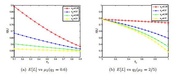
First, we consider the Geo/Geo/1 queueing model, where the system parameters

λ_{0} = 0.3

λ_{1} = 0.5

λ_{2} = 0.6

μ_{1} = 1 / 3

η_{0} = 0.8

η_{1} = 0.3

. Taking different values

η_{2} = 0.35, 0.5, 0.65, 0.8

, Fig. 1(a) and Fig. 1(b) show the impacts of

μ_{2}

and

q_{2}

on the expected number of customers in the system

E [L]

for different values of

η_{2}

, respectively. Obviously, from Fig. 1(a) and Fig. 1(b), the mean queue length decreases with the increase of

μ_{2}

and

q_{2}

. Furthermore, from Fig. 1(a) or Fig. 1(b), if

μ_{2}

and

q_{2}

are fixed, the smaller

η_{2}

is, the larger

E [L]

becomes, which are identical to the intuitive expectations. Additionally, we should note that the smaller of

η_{2}

, the faster decrease of

E [L]

with the increase of

μ_{2}

. On the contrary, the larger of

η_{2}

, the slower decrease of

E [L]

with the increase of

q_{2}

. We also find that as

q_{2}

reaches to 0,

E [L]

tends to a fix value no matter the values of

η_{2}

. It is reasonable that when

q_{2}

approaches to 0, the system reduces to a 2-phase random environment(repair phase and one operating environment), and

η

has no impact on

E [L]

, which also agrees with the intuitive expectation.

Figure 1 $E [L]$ versus $μ_{2}$ and $q_{2}$ for different $η_{2}$ (Geo/Geo/1)

Full size|PPT slide

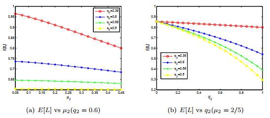
Second, we consider the Geo/NB/1 queueing model, where

S_{1}

is a Pascal distribution with parameters

(2, 2 / 3)

S_{2}

is also a Pascal distribution with parameters

(2, 2 μ_{2})

λ_{0} = 0.3

λ_{1} = 0.5

λ_{2} = 0.6

η_{0} = 0.8

η_{1} = 0.3

. Taking different values

η_{2} = 0.35, 0.5, 0.65, 0.8

, Figure 2(a) and Figure 2(b) show the impacts of

μ_{2}

and

q_{2}

on the expected number of customers in the system

E [L]

for different values of

η_{2}

, respectively. Evidently, Figure 2(a) and Figure 2(b) show that the mean queue length

E [L]

has the same variation tendency as that for the Geo/Geo/1 queue.

Figure 2 $E [L]$ versus $μ_{2}$ and $q_{2}$ for different $η_{2}$ (Geo/NB/1)

Full size|PPT slide

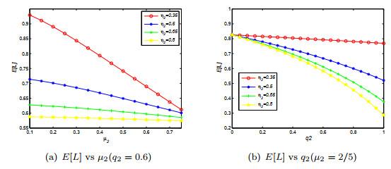
Third, we discuss the Geo/U/1 queueing model, where

S_{1}

is a discrete uniform distribution with parameter 5 and mean 3, (i.e.,

μ_{1} = 1 / 3

), and

S_{2}

is a discrete Uniform distribution with parameter

2 / μ_{2} - 1

and mean

1 / μ_{2}

λ_{0} = 0.3

λ_{1} = 0.5

λ_{2} = 0.6

η_{0} = 0.8

η_{1} = 0.3

. Taking different values

η_{2} = 0.35, 0.5, 0.65, 0.8

, Figure 3(a)and Figure 3(b) show the effects of

μ_{2}

and

q_{2}

on the expected number of customers in the system

E [L]

for different values of

η_{2}

, respectively. From Figure 3(a) and Figure 3(b), it is obviously that for the Geo/U/1 queue, the mean queue length also has the same variation trend.

Figure 3 $E [L]$ versus $μ_{2}$ and $q_{2}$ for different $η_{2}$ (Geo/U/1)

Full size|PPT slide

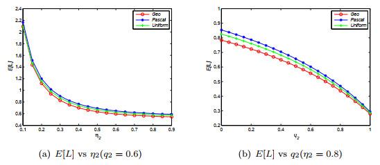
Finally, Figure 4 shows that with the same service rate, different service time distributions have different impacts on the expected number of customers in the system

E [L]

, where

λ_{0} = 0.3

λ_{1} = 0.5

λ_{2} = 0.6

η_{0} = 0.8

η_{1} = 0.3

μ_{1} = 1 / 3

μ_{2} = 2 / 5

. As shown in Figure 4, with the same mean service time, different service time distributions have the different impacts on the mean queue length. The Geo/NB/1 queue has the largest value, the Geo/U/1 queue has the lowest value. Moreover, the overall results confirm that

E [L]

is a decreasing function of

μ_{2}

and

q_{2}

for the three queueing models. The numerical example also implies that if we want to develop a better service, we need to select an appropriate service type.

Figure 4 $E [L]$ versus $η_{2}$ and $q_{2}$ with different service time distributions

Full size|PPT slide

8 Conclusions

This paper discussed a Geo/G/1 queue in a multi-phase service environment with disasters. By using the supplementary variable technique, we defined a Markov process and presented the analytically explicit expressions for the PGF of the queue length distribution at an arbitrary epoch. Some important performance measures such as the expected length of cycle time, the PGF of the stationary sojourn time of an arbitrary customer, and the PGF of the server's working time in a service cycle were obtained. It is noted that the continuous-time M/G/1 queue can be approximated by the discrete-time queue, and we also showed the relationship between the discrete-time system and its continuous-time counterpart. Finally, we provided some examples and numerical results to demonstrate the impacts of parameters on the mean queue length.

References

Publishing order | Descend order by publishing year | Descend order by cited within

1	Yechiali U. Queues with system disasters and impatient customers when system is down. Queueing Systems, 2007, 56, 195- 202. https://doi.org/10.1007/s11134-007-9031-z Cited in this article [1]

2	Giorno V, Nobile A G, Spina S. On some time non-homogeneous queueing systems with catastrophes. Applied Mathematics and Computation, 2014, 245, 220- 234. https://doi.org/10.1016/j.amc.2014.07.076

3	Paz N, Yechiali U. An M/M/1 queue in random environment with disasters. Asia-Pacific Journal of Operational Research, 2014, 31 (3) https://doi.org/10.1142/S021759591450016X

4	Mytalas G C, Zazanis M A. An M^[x]/G/1 queueing system with disasters and repairs under a multiple adapted vacation policy. Naval Research Logistics, 2015, 62, 171- 189. https://doi.org/10.1002/nav.21621

5	Sudhes R, Sebasthi Priya R, Lenin R B. Analysis of N-policy queues with disastrous breakdown. TOP, 2016, 24, 612- 634. https://doi.org/10.1007/s11750-016-0411-6

6	Kapodistria S, Phung-Duc T, Resing J. Linear birth/immigration-death process with binomial catastrophes. Probability in the Engineering and Informational Sciences, 2016, 30 (1): 79- 111. https://doi.org/10.1017/S0269964815000297

7	Jiang T, Liu L. Analysis of a GI/M/1 in a multi-phase service environment with disasters. RAIRO — Operations Research, 2017, 51, 79- 100. https://doi.org/10.1051/ro/2016005

8	Jiang T, Liu L. The GI/M/1 queue in a multi-phase service environment with disasters and working breakdowns. International Journal of Computer Mathematics, 2017, 94 (4): 707- 726. https://doi.org/10.1080/00207160.2015.1128531

9	Zhang X, Liu L, Jiang T. Analysis of an M/G/1 stochastic clearing queue in a 3-Phase Environment. Journal of Systems Science and Information, 2015, 3 (4): 374- 384. https://doi.org/10.1515/JSSI-2015-0374

10	Ye J, Liu L, Jiang T. Analysis of a single-sever queue with disasters and repairs under Bernoulli vacation schedule. Journal of Systems Science and Information, 2016, 4 (6): 547- 559. https://doi.org/10.21078/JSSI-2016-547-13 Cited in this article [1]

11	Atencia I, Moreno P. The discrete-time Geo/Geo/1 queue with negative customers and disasters. Computers & Operations Research, 2004, 31, 1537- 1548. https://www.sciencedirect.com/science/article/abs/pii/S0305054803001072 Cited in this article [1]

12	Yi X W, Kim J D, Choi D W, et al. The Geo/G/1 queue with disasters and multiple working vacations. Stochastic Models, 2007, 23, 21- 31. Cited in this article [1]

13	Park H M, Yang W S, Chae K C. The Geo/G/1 with negative customers and disasters. Stochastic Models, 2009, 25, 673- 688. Cited in this article [1]

14	Park H M, Yang W S, Chae K C. Analysis of the GI/Geo/1 queue with disasters. Stochastic Analyis and Applications, 2010, 28, 44- 53. Cited in this article [1]

15	Lee D H, Yang W S, Park H M. Geo/G/1 queues with disasters and general repair times. Applied Mathematical Modelling, 2011, 35, 1561- 1570. https://doi.org/10.1016/j.apm.2010.09.032 Cited in this article [2]

16	Lee D H, Yang W S. The N-policy of a discrete time Geo/G/1 queue with disasters and its application to wireless sensor networks. Applied Mathematical Modelling, 2013, 37, 9722- 9731. https://doi.org/10.1016/j.apm.2013.05.012 Cited in this article [1]

17	Atencia I, Moreno P. A Discrete-Time Geo/G/1 retrial queue with the server subject to starting failures. Annals of Operations Research, 2006, 141, 85- 107. https://doi.org/10.1007/s10479-006-5295-7 Cited in this article [2]

18	Yang T, Li H. On the steady-state queue size distribution of the discrete-time Geo/G/1 queue with repeated customers. Queueing Systems, 1995, 21, 199- 215. https://doi.org/10.1007/BF01158581 Cited in this article [2]

Funding

the National Natural Science Foundation of China(61773014)

PDF(190 KB)

177

Accesses

Citation

Detail

Sections

Recommended

Abstract
Key words
Cite this article
1 Introduction
2 Model Description
3 Stationary Queue Size Distribution
4 Performance Measures
5 The Length of Working Time in a Cycle
6 Relation to the Continuous-Time System
7 Some Numerical Examples
Figure 1 $E [L]$ versus $μ_{2}$ and $q_{2}$ for different $η_{2}$ (Geo/Geo/1)
Figure 2 $E [L]$ versus $μ_{2}$ and $q_{2}$ for different $η_{2}$ (Geo/NB/1)
Figure 3 $E [L]$ versus $μ_{2}$ and $q_{2}$ for different $η_{2}$ (Geo/U/1)
Figure 4 $E [L]$ versus $η_{2}$ and $q_{2}$ with different service time distributions
8 Conclusions
References
Funding

Received	Accepted	Published
2017-08-24	2017-12-07	2018-08-25
Issue Date
2018-08-25

Please choose a citation manager

Content to export

Abstract

Key words

Cite this article

1 Introduction

2 Model Description

3 Stationary Queue Size Distribution

4 Performance Measures

5 The Length of Working Time in a Cycle

6 Relation to the Continuous-Time System

7 Some Numerical Examples

Figure 1 $E [L]$ versus $μ_{2}$ and $q_{2}$ for different $η_{2}$ (Geo/Geo/1)

Figure 2 $E [L]$ versus $μ_{2}$ and $q_{2}$ for different $η_{2}$ (Geo/NB/1)

Figure 3 $E [L]$ versus $μ_{2}$ and $q_{2}$ for different $η_{2}$ (Geo/U/1)

Figure 4 $E [L]$ versus $η_{2}$ and $q_{2}$ with different service time distributions

8 Conclusions

{{custom_sec.title}}

{{custom_sec.title}}

References

{{custom_fnGroup.title_en}}

Footnotes

Funding

Share

模态框（Modal）标题

Please choose a citation manager

Content to export

Abstract

Key words

Cite this article

1 Introduction

2 Model Description

3 Stationary Queue Size Distribution

4 Performance Measures

5 The Length of Working Time in a Cycle

6 Relation to the Continuous-Time System

7 Some Numerical Examples

Figure 1 E[L] versus μ2 and q2 for different η2 (Geo/Geo/1)

Figure 2 E[L] versus μ2 and q2 for different η2 (Geo/NB/1)

Figure 3 E[L] versus μ2 and q2 for different η2 (Geo/U/1)

Figure 4 E[L] versus η2 and q2 with different service time distributions

8 Conclusions

{{custom_sec.title}}

{{custom_sec.title}}

References

{{custom_fnGroup.title_en}}

Footnotes

Funding

Figure 1 $E [L]$ versus $μ_{2}$ and $q_{2}$ for different $η_{2}$ (Geo/Geo/1)

Figure 2 $E [L]$ versus $μ_{2}$ and $q_{2}$ for different $η_{2}$ (Geo/NB/1)

Figure 3 $E [L]$ versus $μ_{2}$ and $q_{2}$ for different $η_{2}$ (Geo/U/1)

Figure 4 $E [L]$ versus $η_{2}$ and $q_{2}$ with different service time distributions