Non-equidistance DGM(1, 1) Model Based on the Concave Sequence and Its Application to Predict the China's Per Capita Natural Gas Consumption

Xinhai KONG; Yong ZHAO; Jiajia CHEN

doi:10.21078/JSSI-2018-376-09

PDF(154 KB)

Journal of Systems Science and Information ›› 2018, Vol. 6 ›› Issue (4) : 376-384. DOI: 10.21078/JSSI-2018-376-09

Non-equidistance DGM(1, 1) Model Based on the Concave Sequence and Its Application to Predict the China's Per Capita Natural Gas Consumption

Author information +

History +

Abstract

Although the grey forecasting model has been successfully adopted in various fields and demonstrated promising results, the literatures show its performance could be further improved, such as for the DGM(1, 1) model, based on a concave sequence, the modeling error will be larger. In this paper, firstly the definition of sequence convexity is given out, and it is proved that the output sequence of DGM(1, 1) model is a convex sequence. Next, the residual change law of DGM(1, 1) model based on the concave sequence is discussed, and the non-equidistance DGM(1, 1) model is proposed. Finally, by introducing the symmetry transformation, a concave sequence is transformed into a convex sequence, called the symmetric sequence of the concave sequence, and then construct the non-equidistance DGM(1, 1) model based on the convex sequence. The example results show that the novel method is more accurate than the direct modeling for a concave sequence.

Key words

DGM (1, 1) Model / concave sequence / initialization / symmetry transformation / non-equidistance DGM (1, 1) model

Cite this article

EndNote

Ris (Procite)

Bibtex

Download Citations

Xinhai KONG , Yong ZHAO , Jiajia CHEN. Non-equidistance DGM(1, 1) Model Based on the Concave Sequence and Its Application to Predict the China's Per Capita Natural Gas Consumption. Journal of Systems Science and Information, 2018, 6(4): 376-384 https://doi.org/10.21078/JSSI-2018-376-09

1 Introduction

Grey forecasting model is an important part of grey theory, and it is an important tool to deal with small samples and poor information. Xie^[1] proposed the discrete grey model abbreviated as DGM(1, 1) model, and soon to be widely used^[2−5]. But in the actual application process, DGM(1, 1) model with homogeneous exponential characteristic, also can appear that the modeling error is large, so many scholars have proposed a series of optimization measures to extend the application scope of DGM(1, 1) model.

A novel discrete grey model was proposed to suit the inhomogeneous exponential growth law^[6]. Xie^[7] proposed a kind of optimization algorithm of DGM(1, 1) model based on the boundary values and made an empirical research, but Su^[8] has demonstrated that the algorithm maybe cause the deterioration phenomenon of the model relative error, and by using the least square method to reconstruct the DGM(1, 1) model with an optimal boundary value. Yang^[9] provided a novel way to construct the DGM(1, 1) model based on the class ratio sequence of an original sequence, and the predicted values can be realized by forecasting the class ratio sequence. According to the change characteristics of the class ratio sequence, reducing the class ratio dispersion is used to improve the modeling accuracy^[10]. By introducing the translation transformation and geometric mean transformation, another DGM(1, 1) model to suit random oscillation sequences was presented^[11]. According to the principle of new information priority on grey system theory, the DGM(1, 1) forecasting model that

x^{(1)} (n)

is taken as the initial condition was established^[12].

However, no matter which method is used, the output sequence of DGM(1, 1) model is always a convex sequence. If constructing the DGM(1, 1) model based on the concave sequence, it will lead to the inconsistency of growing trend between the forecasting sequence and the original sequence. In order to overcome the model error, this paper presents a novel method. By the symmetry transformation, a concave sequence will be transformed into a convex sequence, and then construct the DGM(1, 1) model based on the convex sequence.

Since the original sequence after the symmetry transformation becomes a non-equidistant sequence, and for the non-equidistance GM(1, 1) model, there has been many research results^[13−19], but the research on non-equidistance DGM(1, 1) model is less. Therefore, according to the non-equidistance GM(1, 1) modeling method, this paper construct a non-equidistance DGM(1, 1) model.

2 The Definition and Property of Concave or Convex Sequences

Definition 1 Assume that

X^{(0)} = {x^{(0)} (1), x^{(0)} (2), \dots, x^{(0)} (n)}

is a given data sequence, if it satisfies

Δ^{(0)} (k) \leq Δ^{(0)} (k - 1)

(

2 \leq k \leq n

), then

X^{(0)}

is called a concave sequence; if it satisfies

Δ^{(0)} (k) \geq Δ^{(0)} (k - 1) (2 \leq k \leq n

), then

X^{(0)}

is called a convex sequence, where

Δ^{(0)} (k) = x^{(0)} (k) - x^{(0)} (k - 1)

. Especially, when

Δ^{(0)} (k) < Δ^{(0)} (k - 1)

(or

Δ^{(0)} (k) > Δ^{(0)} (k - 1)

X^{(0)}

is called a strictly concave sequence (or a strictly convex sequence).

Theorem 1 If $X^{(0)} = {x^{(0)} (1), x^{(0)} (2), \dots, x^{(0)} (n)}$ is a concave sequence or a convex sequence, and then satisfy the inequality

2 x^{(0)} (k) \geq x^{(0)} (k + 1) + x^{(0)} (k - 1)

(1)

2 x^{(0)} (k) \leq x^{(0)} (k + 1) + x^{(0)} (k - 1) .

(2)

Proof If

X^{(0)}

is a concave sequence, from the Definition 1, it follows that

Δ^{(0)} (k) \leq Δ^{(0)} (k - 1)

, that is,

x^{(0)} (k + 1) - x^{(0)} (k) \leq x^{(0)} (k) - x^{(0)} (k - 1)

, such that

2 x^{(0)} (k) \geq x^{(0)} (k + 1) + x^{(0)} (k - 1)

. Especially, when

X^{(0)}

is a strictly concave sequence, Equation (1) does not contain the equal sign. Similarly,

X^{(0)}

is a convex sequence, Equation (2) holds true.

3 The Definition and Property of Concave or Convex Sequences

3.1 Overview of the DGM(1, 1) Model

Definition 2^[1] Assume that

X^{(0)} = {x^{(0)} (1), x^{(0)} (2), \dots, x^{(0)} (n)}

is a nonnegative sequence, and its accumulated generation sequence is denoted as

X^{(1)} = {x^{(1)} (1), x^{(1)} (2), \dots

x^{(1)} (n)}

, where

x^{(1)} (k) = \sum_{m = 1}^{k} x^{(0)} (m)

k = 1, 2, \dots, n

, then the equation

x^{(1)} (k + 1) = β_{1} x^{(1)} (k) + β_{2}

(3)

is called the discrete GM(1, 1) model abbreviated as the DGM(1, 1) model.

According to the least square method, the parameters of DGM(1, 1) model satisfy

\hat{β} = [β_{1}, β_{2}]^{T} = (B^{T} B)^{- 1} B^{T} Y,

(4)

where

B = [\begin{matrix} x^{(1)} (1) & 1 \\ x^{(1)} (2) & 1 \\ ⋮ & ⋮ \\ x^{(1)} (n - 1) & 1 \end{matrix}], Y = [\begin{matrix} x^{(1)} (2) \\ x^{(1)} (3) \\ ⋮ \\ x^{(1)} (n) \end{matrix}],

and then we get

{\begin{aligned} β_{1} & = \frac{\sum_{k = 1}^{n - 1} x^{(1)} (k + 1) x^{(1)} (k) - \frac{1}{n - 1} \sum_{k = 1}^{n - 1} x^{(1)} (k + 1) \sum_{k = 1}^{n - 1} x^{(1)} (k)}{{\sum_{k = 1}^{n - 1} (x^{(1)} (k))}^{2} - \frac{1}{n - 1} {(\sum_{k = 1}^{n - 1} x^{(1)} (k))}^{2}}, \\ β_{2} & = \frac{1}{n - 1} [\sum_{k = 1}^{n - 1} x^{(1)} (k + 1) - β_{1} \sum_{k = 1}^{n - 1} x^{(1)} (k)] . \end{aligned}

(5)

Let

x^{(1)} (1) = x^{(0)} (1)

, from Equation (3), the time response function can easily be deduced as follows

{\hat{x}}^{(1)} (k + 1) = β_{1}^{k} (x^{(0)} (1) - \frac{β_{2}}{1 - β_{1}}) + \frac{β_{2}}{1 - β_{1}}, k = 1, 2, \dots, n - 1.

(6)

Therefore, the restored values of

x^{(0)} (k)

are given by

\begin{aligned} {\hat{x}}^{(0)} (k + 1) & = {\hat{x}}^{(1)} (k + 1) - {\hat{x}}^{(1)} (k) \\ = β_{1}^{k} (x^{(0)} (1) - \frac{β_{2}}{1 - β_{1}}) - β_{1}^{k - 1} (x^{(0)} (1) - \frac{β_{2}}{1 - β_{1}}) \\ = β_{1}^{k - 1} (x^{(0)} (1) - \frac{β_{2}}{1 - β_{1}}) (β_{1} - 1), \end{aligned}

(7)

and its class ratio sequence is defined as

\hat{σ} (k) = \frac{{\hat{x}}^{(0)} (k + 1)}{{\hat{x}}^{(0)} (k)} = β_{1}, k = 1, 2, \dots, n - 1.

For a positive sequence

X = {x^{(0)} (k) | x^{(0)} (k) > 0}

, obviously, its class ratio satisfies

β_{1} > 0

; If

β_{1} = 1

, then

{\hat{x}}^{(0)} (k) = c

, where

c

is a constant.

3.2 The Change Law of Forecasting Sequence of DGM(1, 1) Model

In the use of DGM(1, 1) model, it is usually a sequence of positive numbers, and in this case, the simulated and forecasting sequence of DGM(1, 1) model are usually positive (except for a handful of anomalous data). In this paper, we only discuss the output sequence of DGM(1, 1) model is positive.

Theorem 2 When the output sequence of DGM $(1, 1)$ model is positive, the output sequence is also a convex sequence.

Proof Since the output values of DGM(1, 1) model are all positive, it means the value of Equation (7) is positive in all of

k = 1, 2, \dots, n

, that is

β_{1}^{k - 1} (x^{(0)} (1) - \frac{β_{2}}{1 - β_{1}}) (β_{1} - 1) > 0.

(8)

Considering the incremental sequence

\tilde{Δ} (k) = {\hat{x}}^{(0)} (k + 1) - {\hat{x}}^{(0)} (k) = β_{1}^{k - 2} (x^{(0)} (1) - \frac{β_{2}}{1 - β_{1}}) (β_{1} - 1)^{2}

(9)

and

\tilde{Δ} (k - 1) = {\hat{x}}^{(0)} (k) - {\hat{x}}^{(0)} (k - 1) = β_{1}^{k - 3} (x^{(0)} (1) - \frac{β_{2}}{1 - β_{1}}) (β_{1} - 1)^{2} .

(10)

Let Equation (9) be divided by Equation (10), then

\frac{\tilde{Δ} (k)}{\tilde{Δ} (k - 1)} = \frac{β_{1}^{k - 2} (x^{(0)} (1) - \frac{β_{2}}{1 - β_{1}}) {(β_{1} - 1)}^{2}}{β_{1}^{k - 3} (x^{(0)} (1) - \frac{β_{2}}{1 - β_{1}}) {(β_{1} - 1)}^{2}} = β_{1} .

(11)

1) When

β_{1} > 1

, then

β_{1} - 1 > 0

. From Equation (8), it follows that

x^{(0)} (1) - \frac{β_{2}}{1 - β_{1}} > 0

. According to Equation (9), we know that

\tilde{Δ} (k) > 0

, obviously there exists

{\hat{x}}^{(0)} (k + 1) \geq {\hat{x}}^{(0)} (k)

and

\tilde{Δ} (k) > \tilde{Δ} (k - 1)

. That is, the simulative and forecasting sequence is a monotone increasing convex sequence.

2) When

0 < β_{1} < 1

, then

β_{1} - 1 < 0

. From Equation (8), it follows that

x^{(0)} (1) - \frac{β_{2}}{1 - β_{1}} < 0

. According to Equation (9), we know that

\tilde{Δ} (k) < 0

, obviously there exist

{\hat{x}}^{(0)} (k + 1) \leq {\hat{x}}^{(0)} (k)

and

\tilde{Δ} (k) > \tilde{Δ} (k - 1)

. That is, the simulative and forecasting sequence is a monotone decreasing convex sequence.

Theorem 2 shows that the restored sequence of DGM(1, 1) model is actually a convex sequence, and for a concave sequence, the DGM(1, 1) modeling will produce large errors. As shown in Figure 1, when the original sequence is a concave sequence, the geometrical shape of the output sequence obtained by Equation (3) is inconsistent with the original sequence.

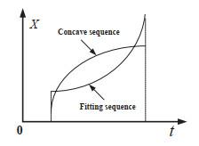
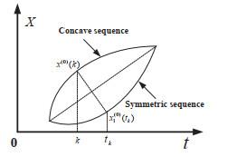
Figure 1 The growing trend of fitting sequence of DGM(1, 1) model

Full size|PPT slide

4 The Symmetry Transformation of a Concave Sequence

As the above analysis shows that as long as put on a convex sequence into a concave sequence can avoid the model error. The symmetry transformation is the most effective way to change the convexity of a sequence, which is to take the straight line through the first point and the

n

-th point as the axis of symmetry (see Figure 2). In order to eliminate the influence of the dimensions, the original sequence is processed, i.e.,

x_{0}^{(0)} (k) = \frac{x^{(0)} (k)}{x^{(0)} (1)}

. Therefore, we can obtain the initialization sequence denoted as

X_{0}^{(0)} = {x_{0}^{(0)} (1), x_{0}^{(0)} (2), \dots, x_{0}^{(0)} (n)}

Figure 2 The symmetry transformation of a concave sequence

Full size|PPT slide

Theorem 3 Assume that $X^{(0)} = {x^{(0)} (1), x^{(0)} (2), \dots, x^{(0)} (n)}$ is a positive sequence, and $X_{0}^{(0)}$ is the initialization sequence of $X^{(0)}$ , carry out the symmetry transformation with regard to $X_{0}^{(0)}$ , then we get the convex sequence denoted as $X_{1}^{(0)} = {x_{1}^{(0)} (t_{1}), x_{1}^{(0)} (t_{2}), \dots, x_{1}^{(0)} (t_{n})}$ , where

{\begin{array}{lll} d x_{1}^{(0)} (t_{k}) = \frac{2 (k - 1) (n - 1) (x_{0}^{(0)} (n) - x_{0}^{(0)} (1)) + 2 x_{0}^{(0)} (1) {(n - 1)}^{2} + [{(x_{0}^{(0)} (n) - x_{0}^{(0)} (1))}^{2} - {(n - 1)}^{2}] x_{0}^{(0)} (k)}{{(n - 1)}^{2} + {(x_{0}^{(0)} (n) - x_{0}^{(0)} (1))}^{2}}, \\ d t_{k} = k + \frac{x_{0}^{(0)} (n) - x_{0}^{(0)} (1)}{n - 1} (x_{0}^{(0)} (k) - x_{0}^{(0)} (t_{k})) . \end{array}

(12)

Proof Based on the two-point method, the linear equation of the axis of symmetry is given by

\frac{x - x_{0}^{(0)} (1)}{x_{0}^{(0)} (n) - x_{0}^{(0)} (1)} = \frac{t - 1}{n - 1} .

(13)

For any point

(k, x_{0}^{(0)} (k))

, and its symmetry point denoted by

(t_{k}, x_{1}^{(0)} (t_{k}))

, then the center of two points satisfies Equation (13), namely

\frac{\frac{x_{0}^{(0)} (k) + x_{1}^{(0)} (t_{k})}{2} - x_{0}^{(0)} (1)}{x_{0}^{(0)} (n) - x_{0}^{(0)} (1)} = \frac{\frac{k + t_{k}}{2} - 1}{n - 1} .

(14)

According to the product of two vertical slope is

- 1

, it follows that

(\frac{x_{0}^{(0)} (n) - x_{0}^{(0)} (1)}{n - 1}) (\frac{x_{0}^{(0)} (k) - x_{1}^{(0)} (t_{k})}{k - t_{k}}) = - 1.

(15)

Combining Equation (14) and Equation (15), we can get the new values in Equation (12).

Obviously, when

k = 1

, we have

x_{1}^{(0)} (t_{1}) = x_{0}^{(0)} (1)

; When

k = n

, we have

x_{1}^{(0)} (t_{n}) = x_{0}^{(0)} (n)

For an original concave sequence after the symmetry transformation, since

Δ t_{k}

(Δ t_{k} = t_{k} - t_{k - 1})

is not a constant, the symmetry transformation sequence is a non-equidistant sequence. So it is necessary to establish the non-equidistant DGM(1, 1) model.

5 The Non-Equidistant DGM(1, 1) Model Based on the Concave Sequence

5.1 The Principle of the Non-Equidistant DGM(1, 1) Model

Definition 3 Assume that

X^{(0)} = {x^{(0)} (t_{1}), x^{(0)} (t_{2}), \dots, x^{(0)} (t_{n})}

is a nonnegative sequence, and

X^{(1)} = {x^{(1)} (t_{1}), x^{(1)} (t_{2}), \dots, x^{(1)} (t_{n})}

is the first accumulated generation sequence, where

x^{(1)} (k) = \sum_{i = 1}^{k} Δ t_{i} x^{(0)} (i)

Δ t_{1} = 1

Δ t_{i} = t_{i} - t_{i - 1}

i = 2, \dots, n

k = 1, 2, \dots, n

, the equation

x^{(1)} (t_{k + 1}) = β_{1} x^{(1)} (t_{k}) + β_{2}

(16)

is called the non-equidistant discrete grey model, abbreviated as the non-equidistant DGM(1, 1) model.

By the least square method, the parameters in the non-equidistant DGM(1, 1) model satisfy

\hat{β} = [β_{1}, β_{2}]^{T} = (B^{T} B)^{- 1} B^{T} Y

, where

B = [\begin{matrix} x^{(1)} (t_{1}) & 1 \\ x^{(1)} (t_{2}) & 1 \\ ⋮ & ⋮ \\ x^{(1)} (t_{n - 1}) & 1 \end{matrix}], Y = [\begin{matrix} x^{(1)} (t_{2}) \\ x^{(1)} (t_{3}) \\ ⋮ \\ x^{(1)} (t_{n}) \end{matrix}] .

(17)

Namely,

{\begin{aligned} β_{1} & = \frac{\sum_{k = 1}^{n - 1} x^{(1)} (t_{k + 1}) x^{(1)} (t_{k}) - \frac{1}{n - 1} \sum_{k = 1}^{n - 1} x^{(1)} (t_{k + 1}) \sum_{k = 1}^{n - 1} x^{(1)} (t_{k})}{{\sum_{k = 1}^{n - 1} (x^{(1)} (t_{k}))}^{2} - \frac{1}{n - 1} {(\sum_{k = 1}^{n - 1} x^{(1)} (t_{k}))}^{2}}, \\ β_{2} & = \frac{1}{n - 1} [\sum_{k = 1}^{n - 1} x^{(1)} (t_{k + 1}) - β_{1} \sum_{k = 1}^{n - 1} x^{(1)} (t_{k})] . \end{aligned}

(18)

Let

x^{(1)} (1) = x^{(0)} (1)

, the time recursive function is given by

{\hat{x}}^{(1)} (t_{k + 1}) = β_{1}^{k} (x^{(0)} (t_{1}) - \frac{β_{2}}{1 - β_{1}}) + \frac{β_{2}}{1 - β_{1}}, k = 1, 2, \dots,

(19)

and then the restored values or forecasting sequence can be given by

{\hat{x}}^{(0)} (t_{k + 1}) = \frac{{\hat{x}}^{(1)} (t_{k + 1}) - {\hat{x}}^{(1)} (t_{k})}{Δ t_{k + 1}}, k = 1, 2, \dots .

(20)

The difference between the non-equidistant DGM(1, 1) model and the DGM(1, 1) model can be summarized as follows.

1) The data interval. For any

k = 2, 3, \dots, n

Δ t_{k} = t_{k} - t_{k - 1} = c

(

c

is a constant)in the definition of DGM(1, 1) model.

2) The accumulation way. As we know that the accumulated generation sequence of the equidistant DGM(1, 1) model is defined as

x^{(1)} (k) = \sum_{i = 1}^{k} x^{(0)} (i)

k = 1, 2, \dots, n

, but the accumulated generation sequence of the non-equidistant DGM(1, 1) model is defined as

x^{(1)} (t_{k}) = \sum_{i = 1}^{k} Δ t_{i} x^{(0)} (t_{i})

3) The time response function. Compared Equation (6) with Equation (19), both are the same in form.

4) The restored method. From Equation (7) and Equation (20), we can see that the two restored methods are different; this is caused by different accumulating ways.

5.2 The Non-Equidistant DGM(1, 1) Model Based on the Concave Sequence

In order to establish the DGM(1, 1) model for a concave sequence, firstly, the original sequence is processed by initialization, and then carry out the symmetric transformation and use the symmetric sequence to establish a non-equidistant DGM(1, 1) model. Finally, we should do the inverse transformation to restore. The specific algorithm flow as follows.

Step 1 For a positive concave sequence

X^{(0)} = {x^{(0)} (1), x^{(0)} (2), \dots, x^{(0)} (n)}

, by means of initialization, we can get the initialization sequence

X_{0}^{(0)}

Step 2 Use Equation (12) to calculate the symmetry point

(t_{k}, x_{1}^{(0)} (t_{k}))

k = 1, 2, \dots, n

Step 3 Establish the non-equidistant DGM(1, 1) model based on the symmetric sequence

X_{1}^{(0)}

, we can get the fitting sequence

{\hat{X}}_{1}^{(0)} = {{\hat{x}}_{1}^{(0)} (t_{k})}

Step 4 Use Equation (12) to do the inverse transformation, and then we will obtain the fitting sequence of

X_{0}^{(0)}

denoted by

{\hat{X}}_{0}^{(0)} = {{\hat{x}}_{0}^{(0)} (k)}

Step 5 Finally calculate the restored values or forecasting sequence

{\hat{x}}^{(0)} (k) = {\hat{x}}_{0}^{(0)} (k) x^{(0)} (1)

(k = 2, 3, \dots)

6 An Application to Predict the China's per Capita Natural Gas Consumption

China's per capita natural gas consumption from 2009 to 2015 are calculated as

X (0) = 13.3, 17.0, 19.7, 21.3, 23.8, 25.1, 26.2

, unit: m

^{3}

. This is a monotone increasing concave sequence. We construct the DGM(1, 1) model based on the raw data and the non-equidistant DGM(1, 1) model with its symmetric sequence respectively, the simulation results are shown in Table 1 and the predicted values are shown in Table 2.

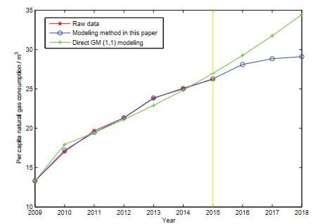
Table 1 Simulated results of two models from 2009 to 2015

Year	Raw data	DGM(1, 1) model			The method in this paper
Year	Raw data	Simulated value	Relative error (%)	Initialization sequence	Symmetric sequence	Gap	Simulated value	Relative error (%)
2009	13.3	13.3000	0	1.0000	1.0000	1.0000	13.3000	0
2010	17.0	17.9252	5.4421	1.2782	1.0510	1.0367	17.2013	1.1842
2011	19.7	19.4497	1.2706	1.4812	1.1735	1.0130	19.4560	1.2384
2012	21.3	21.1039	0.9207	1.6015	1.3744	0.9870	21.3329	0.1544
2013	23.8	22.8988	3.7866	1.7895	1.5110	1.0083	23.8498	0.2091
2014	25.1	24.8463	1.0106	1.8872	1.7333	0.9799	24.9898	0.4390
2015	26.2	26.9595	2.8989	1.9699	1.5556	0.9751	26.2836	0.3190
Average relativeerror (%)			2.1899					0.5063

Table 2 Predicted values of two models from 2016 to 2018

Year	Predicted values of DGM(1, 1) model	Predicted values of the method in this paper (Δt_k = 1)
2016	29.2524	28.0965
2017	31.7404	28.8223
2018	34.4399	29.0962

It can be seen from Table 1, the average relative error of modeling method in this paper is significantly less than that of direct DGM(1, 1) modeling with the raw data, and Figure 3 can directly reflect the fitting effects. It can be also seen from Figure 3 that the predicted values of the modeling method accords with the development trend of the original sequence.

Figure 3 Fitting effects of two models based on the monotone increasing concave sequence

Full size|PPT slide

7 Conclusions

By using the DGM(1, 1) model to forecast a concave sequence, only to optimize the DGM(1, 1) model itself, it is not sure to improve the forecasting accuracy, and even possible the model error becomes large, this is because the forecasting sequence of DGM(1, 1) model is a convex sequence. In this paper, through introducing the symmetric transformation, a concave sequence is transformed into a convex sequence and then we construct the non-equidistant DGM(1, 1) model by using the symmetric sequence (a convex sequence). Thus, the error caused by the grey model is solved fundamentally.

References

Publishing order | Descend order by publishing year | Descend order by cited within

1	Xie N M, Liu S F. Discrete GM(1, 1) and mechanism of grey forecasting model. Systems Engineering — Theory & Practice, 2005, 25 (1): 93- 99. http://en.cnki.com.cn/Article_en/CJFDTOTAL-XTLL200501014.htm Cited in this article [2]

2	Wu X M, Chi D C, Pan X C, et al. Waterlogging prediction based on the discrete grey DGM(1, 1) prediction model. Journal of Shenyang Agricultural University, 2013, 44 (1): 104- 107. Cited in this article [1]

3	Yang L, W S, Dong J P. Grey DGM(1, 1) dynamic prediction model of regional minimum night flow. South-to-North Water Transfers and Water Science & Technology, 2013, 11 (2): 41- 44.

4	Dai T D, Huang X M, Liu H, et al. Research on simulation of convergent deformation of highway tunnel surrounding rock by using DGM(1, 1) model. Central South Highway Engineering, 2013, 38 (6): 102- 105.

5	Liu J F, Liu S F, Fang Z G. Reliability growth evaluation model of binomial system based on DGM(1, 1). China Mechanical Engineering, 2014, 25 (8): 1092- 1095. https://doi.org/10.3969/j.issn.1004-132X.2014.08.019 Cited in this article [1]

6	Xie N M, Liu S F. Research on extension of discrete grey model and its optimize formula. Systems Engineering — Theory & Practice, 2006, 26 (6): 108- 112. Cited in this article [1]

7	Xie N M, Liu S F. Discrete grey forecasting model and its optimization. Applied Mathematical Modelling, 2009, 33 (2): 1173- 1186. https://www.sciencedirect.com/science/article/pii/S0307904X08000206 Cited in this article [1]

8	Su X N, Xie F J. The properties of model DGM(1, 1) and its application in technology innovation. Systems Engineering — Theory & Practice, 2016, 36 (3): 635- 641. http://en.cnki.com.cn/Article_en/CJFDTotal-XTLL201603009.htm Cited in this article [1]

9	Yang B H, Fang Z G, Zhang K. Discrete GM(1, 1) model based on sequence of stepwise ratio. Systems Engineering and Electronics, 2012, 34 (4): 715- 718. Cited in this article [1]

10	Kong X H, Liu Z B, Wei Y. Discrete transform based on monotone decreasing sequence and grey modeling. Statistics and Decision, 2012, (10): 19- 21. Cited in this article [1]

11	Yang F, Guan Y Q, Zeng B, et al. Modeling of DGM(1, 1) based on random oscillatory sequences and its application. Mathematics in Practice and Theory, 2013, (16): 175- 180. Cited in this article [1]

12	Hu P. The DGM(1, 1) model that x⁽¹⁾(n) be taken as initial value. Mathematics in Practice and Theory, 2016, (17): 218- 222. Cited in this article [1]

13	Dai W Z, Li J F. Modeling research on non-equidistance GM(1, 1) model. Systems Engineering — Theory & Practice, 2005, (9): 89- 93. Cited in this article [1]

14	Li L, Li M. GM(1, 1) model of non-isometric time sequence and its application on economy forecast. Journal of Nanjing University of Finance and Economics, 2006, (5): 55- 57.

15	Jiang F, Zheng Y H, Liang R. Method for corrosion risers remaining life prediction based on improved non-equidistant GM(1, 1) model. China Safety Science Journal, 2014, 24 (16): 57- 61.

16	Kang X Q, Wei Y. A new optimized method of non-equigap GM(1, 1) model. The Journal of Grey System, 2008, 20 (4): 373- 384. https://doi.org/10.1002/jgt.20273

17	Wang Y M, Dang Y G, Wang Z X. The optimization of background value in non-equidistant GM(1, 1) model. Chinese Journal of Management Science, 2008, 16 (4): 159- 162.

18	Cui L Z, Liu S F, Wu Z P. The optimization of time response function of the non-equidistance GM(1, 1) model. Statistics and Decision, 2009, (13): 9- 10.

19	Zhang L S, Wang F X. Optimizes grey derivative of unequal interval grey GM(1, 1) model. Mathematics in Practice and Theory, 2010, 40 (11): 63- 67. Cited in this article [1]

20	National Bureau of Statistics of the People's Republic of China. China Statistical Yearbook. Beijing: China Statistics Press, 2016.

Funding

the Natural Fund of Education Department of Sichuan Province(14ZB0388)

the Key Topic of Oil and Gas Development Research Center of Sichuan Province(SKA-02)

PDF(154 KB)

146

Accesses

Citation

Detail

Sections

Recommended

Abstract
Key words
Cite this article
1 Introduction
2 The Definition and Property of Concave or Convex Sequences
3 The Definition and Property of Concave or Convex Sequences
3.1 Overview of the DGM(1, 1) Model
3.2 The Change Law of Forecasting Sequence of DGM(1, 1) Model
Figure 1 The growing trend of fitting sequence of DGM(1, 1) model
4 The Symmetry Transformation of a Concave Sequence
Figure 2 The symmetry transformation of a concave sequence
5 The Non-Equidistant DGM(1, 1) Model Based on the Concave Sequence
5.1 The Principle of the Non-Equidistant DGM(1, 1) Model
5.2 The Non-Equidistant DGM(1, 1) Model Based on the Concave Sequence
6 An Application to Predict the China's per Capita Natural Gas Consumption
Table 1 Simulated results of two models from 2009 to 2015
Table 2 Predicted values of two models from 2016 to 2018
Figure 3 Fitting effects of two models based on the monotone increasing concave sequence
7 Conclusions
References
Funding

Received	Accepted	Published
2017-09-07	2017-12-07	2018-08-25
Issue Date
2018-08-25

Please choose a citation manager

Content to export

Abstract

Key words

Cite this article

1 Introduction

2 The Definition and Property of Concave or Convex Sequences

3 The Definition and Property of Concave or Convex Sequences

3.1 Overview of the DGM(1, 1) Model

3.2 The Change Law of Forecasting Sequence of DGM(1, 1) Model

Figure 1 The growing trend of fitting sequence of DGM(1, 1) model

4 The Symmetry Transformation of a Concave Sequence

Figure 2 The symmetry transformation of a concave sequence

5 The Non-Equidistant DGM(1, 1) Model Based on the Concave Sequence

5.1 The Principle of the Non-Equidistant DGM(1, 1) Model

5.2 The Non-Equidistant DGM(1, 1) Model Based on the Concave Sequence

6 An Application to Predict the China's per Capita Natural Gas Consumption

Table 1 Simulated results of two models from 2009 to 2015

Table 2 Predicted values of two models from 2016 to 2018

Figure 3 Fitting effects of two models based on the monotone increasing concave sequence

7 Conclusions

{{custom_sec.title}}

{{custom_sec.title}}

References

{{custom_fnGroup.title_en}}

Footnotes

Funding

Share

模态框（Modal）标题

Please choose a citation manager

Content to export

Abstract

Key words

Cite this article

1 Introduction

2 The Definition and Property of Concave or Convex Sequences

3 The Definition and Property of Concave or Convex Sequences

3.1 Overview of the DGM(1, 1) Model

3.2 The Change Law of Forecasting Sequence of DGM(1, 1) Model

Figure 1 The growing trend of fitting sequence of DGM(1, 1) model

4 The Symmetry Transformation of a Concave Sequence

Figure 2 The symmetry transformation of a concave sequence

5 The Non-Equidistant DGM(1, 1) Model Based on the Concave Sequence

5.1 The Principle of the Non-Equidistant DGM(1, 1) Model

5.2 The Non-Equidistant DGM(1, 1) Model Based on the Concave Sequence

6 An Application to Predict the China's per Capita Natural Gas Consumption

Table 1 Simulated results of two models from 2009 to 2015

Table 2 Predicted values of two models from 2016 to 2018

Figure 3 Fitting effects of two models based on the monotone increasing concave sequence

7 Conclusions

{{custom_sec.title}}

{{custom_sec.title}}

References

{{custom_fnGroup.title_en}}

Footnotes

Funding