A Modified Gravity p-Median Model for Optimizing Facility Locations

Zhuolin TAO; Qingjing ZHENG; Hui KONG

doi:10.21078/JSSI-2018-421-14

PDF(811 KB)

Journal of Systems Science and Information ›› 2018, Vol. 6 ›› Issue (5) : 421-434. DOI: 10.21078/JSSI-2018-421-14

A Modified Gravity p-Median Model for Optimizing Facility Locations

Author information +

History +

Abstract

The gravity p-median model is an important improvement to the widely-used p-median model. However, there is still a debate on its validity in empirical applications. Previous studies even doubt the significance of the gravity p-median model. Using a case study of tertiary hospitals in Shenzhen, China, this study re-examines the difference between the gravity p-median model with the p-median model, by decomposing the difference between the two models into gravity rule and variant attraction. This study also proposes a modified gravity p-median model by incorporating a distance threshold. The empirical results support the validity of the gravity p-median model, and also reveal that only when the attractions of candidate facility locations are variable will the gravity p-median model lead to different results with the p-median model. The difference between the modified gravity p-median model and the gravity p-median model is also examined. Moreover, the impacts of the distance-decay parameter and distance threshold on solutions are investigated. Results indicate that a larger distance-decay parameter tends to result in a more dispersed distribution of optimal facilities and a smaller average travel time, and a smaller distance threshold can better promote the spatial equity of facilities. The proposed method can also be applied in studies of other types of facilities or in other areas.

Key words

location-allocation / spatial optimization / gravity p-median / distance threshold / Shenzhen

Cite this article

EndNote

Ris (Procite)

Bibtex

Download Citations

Zhuolin TAO , Qingjing ZHENG , Hui KONG. A Modified Gravity p-Median Model for Optimizing Facility Locations. Journal of Systems Science and Information, 2018, 6(5): 421-434 https://doi.org/10.21078/JSSI-2018-421-14

1 Introduction

Location-allocation models are among the most efficient and widely-used methods for optimizing public facility locations, and bunches of models have been developed over the past several decades^[1]. The classic location-allocation models contain four types: The

p

-median problem, the maximum covering location problem (MCLP), the location set covering problem (LSCP), and the

p

-center problem^[2–5]. Among these models, the most popular one is the

p

-median model aiming at minimizing the total or average travel cost (distance/time) from population groups to facilities^[6–8].

A fundamental assumption of the traditional

p

-median model is that each demander only selects the nearest facility to minimize the total travel cost. This assumption requires some preconditions, such as policy restrictions on demanders' selection of facilities, or complete information about facilities' service quality and distances from demanders that enable demanders to make rational selection^{[6, 7]}. In reality, however, this assumption may be inappropriate in some cases, thus the results of the traditional

p

-median model may be biased^[6]. Moreover, in empirical applications, each demand node may contain hundreds or thousands of demanders, making the assumption that all demanders at a node only select the nearest facility more infeasible.

Drezner, et al. developed the gravity

p

-median model^[6] by incorporating the gravity rule into the

p

-median model. The nearest facility assumption is replaced by a gravity-based rule that demanders at each node can select from multiple facilities, and the probability of a demander selecting a facility depends on the facility's attraction and distance from the demander.

However, applications of the gravity

p

-median model are limited. Moreover, no consensus has been reached on its validity in empirical applications. Drezner, et al.^[6] tested the model using a computational experiment, and reached excellent results. By contrast, Carling et al. empirically tested the gravity

p

-median model and compared it with the traditional

p

-median model using three cases, concluding that the gravity

p

-median model leads to similar results with the

p

-median model and thus is of limited use^[7]. Thus, the first objective of this study is to re-examine the validity of the gravity

p

-median model with further empirical evidence. By decomposing the difference between the gravity

p

-median model and

p

-median model into gravity rule and variant attraction, this study provides insights into the mechanism of the gravity

p

-median model, as well as why and when the gravity

p

-median model will lead to different results.

The second objective of this study is to modify the gravity

p

-median model with a distance threshold (i.e., a maximum distance threshold). Previous studies, including some location-allocation models such as MCLP and LSCP^[2], as well as the widely-used two-step floating catchment area (2SFCA) method for modelling spatial accessibility^{[9, 10]}, have argued that a maximum distance should exist. However, the existing gravity rule assumes that there is no restriction on the maximum distance that a facility can provide services^{[6, 7]}. The adoption of a distance threshold in this study makes the assumption of facility selection more realistic and reasonable.

In addition, to improve the accuracy of travel distance/time estimation, the Transit Searching Application Programming Interface (API) and the Driving Searching API developed by Baidu Map are utilized to estimate travel time by transit system or by driving respectively. By using these APIs, the estimation of travel time can take into account multiple transportation modes as well as actual traffic conditions.

Through a case study of tertiary hospitals in Shenzhen, China, this paper provides empirical evidence to enrich the discussion on the empirical validity of the gravity

p

-median model and the proposed modified gravity

p

-median. The findings also have empirical implications to the decision-making of tertiary hospitals planning in Shenzhen.

2 Methodology

2.1 The $p$ -Median Model

The

p

-median model (PM) was first proposed by Hakimi^[4], and is considered as the beginning of location-allocation models^[2]. PM selects a certain number (denoted by

P

) of facility locations from a set of candidate locations, with an objective to minimize the total travel distance from all demanders to the nearest facilities. It can be formulated as:

\begin{array}{rcl} min & \sum_{i} \sum_{j} h_{i} d_{i j} Y_{i j} \end{array}

(1)

\begin{array}{rcl} s . t . & \sum_{j} X_{j} = P, \forall j, \end{array}

(2)

\begin{array}{rcl} \sum_{j} Y_{i j} = 1, \forall i, \end{array}

(3)

\begin{array}{rcl} Y_{i j} - X_{j} \leq 0, \forall i, j, \end{array}

(4)

\begin{array}{rcl} X_{j}, Y_{i j} \in {0, 1}, \forall i, j, \end{array}

(5)

where

i

is the demand node,

j

is the candidate facility location,

h_{i}

is the amount of demanders at node

i

d_{i j}

is travel distance/time from demand node

i

to location

j

, and

P

is the number of facilities to be allocated.

X_{j}

and

Y_{i j}

are decision variables. If candidate location

j

is selected to allocate a facility,

X_{j} = 1

; otherwise,

X_{j} = 0

. If demand node

i

is served by candidate location

j

, that is,

j

is the nearest candidate location from

i

Y_{i j} = 1

; otherwise,

Y_{i j} = 0

2.2 The Gravity $p$ -Median Model

The gravity

p

-median model proposed by Drezner, et al. incorporates the gravity rule into the

p

-median model^[6]. According to the gravity rule, demanders at a demand node select from all facilities rather than only choose the nearest facility. The probability of a demander selecting a facility is positively related to the facility's attraction and negatively related to the distance between them, which can be expressed as:

\begin{array}{rcl} f_{i j} = \frac{S_{j} {d_{i j}}^{- β}}{\sum_{j \in P} S_{j} {d_{i j}}^{- β}}, \end{array}

(6)

where

f_{i j}

is the probability that demanders at node

i

select facility

j

S_{j}

is the attraction of facility

j

d_{i j}

is the travel distance/time from demand node

i

to location

j

β

is the distance-decay parameter of the gravity model, and

P

is the set of selected locations, which contains the candidate locations that are selected in the optimization result. The total number of facility locations in set

P

p

. The distance-decay function adopts a power function form, which is widely used in applications.

Denote the amount of demanders at demand node

i

D_{i}

, then the amount of the part of demanders at node

i

which select facility location

j

can be calculated as:

\begin{array}{rcl} h_{i j} = D_{i} f_{i j} = D_{i} \frac{S_{j} {d_{i j}}^{- β}}{\sum_{j \in P} S_{j} {d_{i j}}^{- β}} . \end{array}

(7)

Finally, we can obtain the total travel distance of all demanders by multiplying

h_{i j}

by the travel distance

d_{i j}

and summing them up:

\begin{array}{rcl} f (P) = \sum_{i} \sum_{j \in P} d_{i j} h_{i j} = \sum_{i} \sum_{j \in P} d_{i j} D_{i} \frac{S_{j} {d_{i j}}^{- β}}{\sum_{j \in P} S_{j} {d_{i j}}^{- β}}, \end{array}

(8)

where

f (P)

is the total travel distance corresponding to selected candidate facility location set

P

. The objective of GPM is to find an optimal set

P

that minimizes

f (P)

2.3 The Modified Gravity $p$ -Median Model

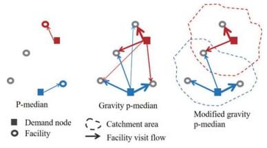
In this study, we propose a modified gravity

p

-median (MGPM) model. MGPM improves GPM by incorporating a maximum travel distance threshold. In other word, compared to GPM, the MGPM further includes an additional constraint of maximum travel distance on the distance-decay function. The difference in facility selection assumptions among the

p

-median, gravity

p

-median and modified gravity

p

-median model can be explicitly illustrated by Figure 1. The line width of arrow to a facility denotes the relative probability of it being selected.

Figure 1 Schematic diagram of three models

Full size|PPT slide

The probability of selecting a facility in MGPM can be expressed as:

\begin{array}{rcl} f_{i j} = \frac{S_{j} {d_{i j}}^{- β}}{\sum_{l \in P ⋂ {k | d_{l k} \leq r}} S_{l} {d_{i l}}^{- β}}, \end{array}

(9)

where

r

is the maximum travel distance threshold or catchment area of facilities,

{k | d_{l k} \leq r}

is the set of facility locations whose distances from demand node

i

are less than or equal to

r

, and the operator

⋂

means location

l

must simultaneously belong to set

P

and

{k | d_{l k} \leq r}

. Other variables are the same with formula (6).

Accordingly, the total travel distance from all demanders to facilities can be calculated as:

\begin{array}{rcl} f (P) = \sum_{i \in {k | d_{k j} \leq r}} \sum_{j \in P ⋂ {k | d_{i k} \leq r}} d_{i j} D_{i} f_{i j}, \end{array}

(10)

where

f (P)

is the total travel distance corresponding to selected facility location set

P

, and

f_{i j}

is defined by formula (9). Similar to GPM, the objective of MGPM is to find an optimal set

P

that minimizes

f (P)

3 Data and Calculation

3.1 Study Area

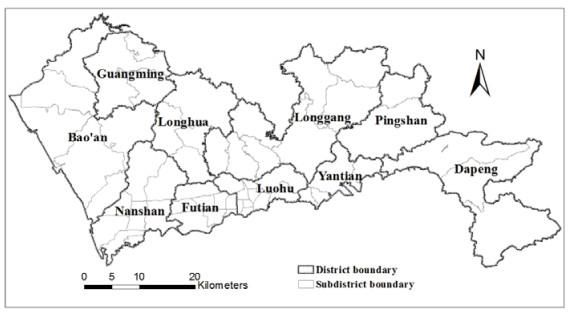
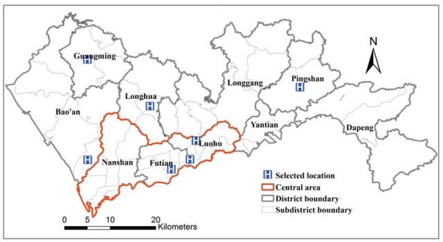
Shenzhen is a coastal city located in Guangdong Province, China. It is one of the core cities in the Pearl River Delta, which is one of the most developed regions in China and one of the largest mega-regions around the world. Shenzhen is now a megacity with 10.78 million permanent population and an administrative area of 1997 square kilometers. There are 10 administrative districts in Shenzhen, including Luohu, Futian, Nanshan, Yantian, Bao'an, Longgang, Guangming, Longhua, Pingshan, and Dapeng, and 55 subdistrict units (Figure 2). Luohu, Futian and Nanshan are the most developed and populous districts in Shenzhen.

Figure 2 Administrative divisions in Shenzhen

Full size|PPT slide

3.2 Data Source of Population and Tertiary Hospitals

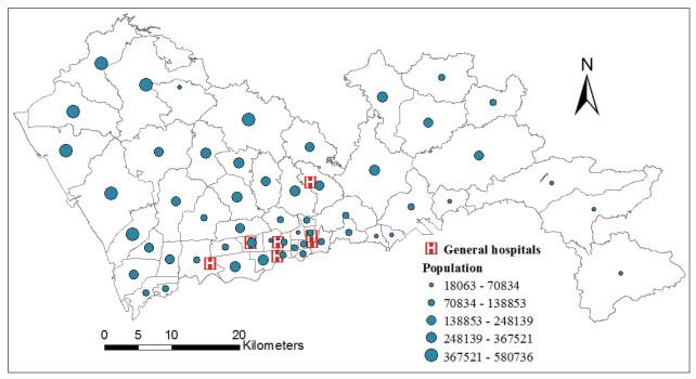
The population data at the subdistrict level used in this study is from the 6th population census data of China at 2010, which is the latest official population census data at the subdistrict level. Due to the lack of population data at a finer scale, the geometry centroids of subdistricts are considered as the demand nodes (Figure 3).

Figure 3 Distribution of population and tertiary hospitals in Shenzhen

Full size|PPT slide

List and addresses of the tertiary hospitals in Shenzhen are obtained from the official website of Shenzhen government (http://www.sz.gov.cn/ylwslyfwzt/kbjy/yljg/). Our latest access to the website was on July 8, 2016. Only the tertiary hospitals are taken into account in this study, because only the tertiary hospitals can be utilized by demanders from all regions in Shenzhen. Other hospitals, such as the district-owned hospitals, are available only at local scale. Moreover, the relatively small quantity of tertiary hospitals is more convenient for the analysis and comparison of results. As shown in Figure 3, there are 7 tertiary hospitals in Shenzhen.

3.3 Travel Time Estimation

Various measures of travel distance have been adopted in existing studies. The travel time measure seems to be the most superior measure of the actual spatial impedance between demanders and facilities, which not only reflects the absolute spatial distance between two sites^{[11, 12]}, but also depends on transportation availability. With the development of geographic information system, the estimation of travel time measure has become convenient^{[13, 14]}.

Most studies estimate travel time by setting a driving speed to each rank of roads, then using network analysis tools to calculate the minimum travel time between any two sites. A common tool is the OD matrix tool in Network Analysis toolbox of ArcGIS. Driving speed is often set according to technical limitation of each rank of roads or actual driving speed^{[13, 14]}. One shortage of this method is that the accuracy of estimation depends on the driving speed, which is somewhat arbitrary in practice. Moreover, the road network data available to individual researcher is often outdated^[15].

Recently, some studies have introduced APIs of online maps such as Google Map or Baidu Map to estimate travel time^[15–17]. In this way, researchers can make use of the dynamically updated transportation network data and the routing rules maintained by map developers to obtain reliable estimation of travel time^[15].

This study utilizes Baidu Map API (lbsyun.baidu.com/index.php) by programming in Java Script to batch estimating travel time from demand nodes to facility locations. Two independent APIs, the Transit Searching API and the Driving Searching API, have been developed by Baidu Map to estimate travel time by transit system or by driving private car respectively. 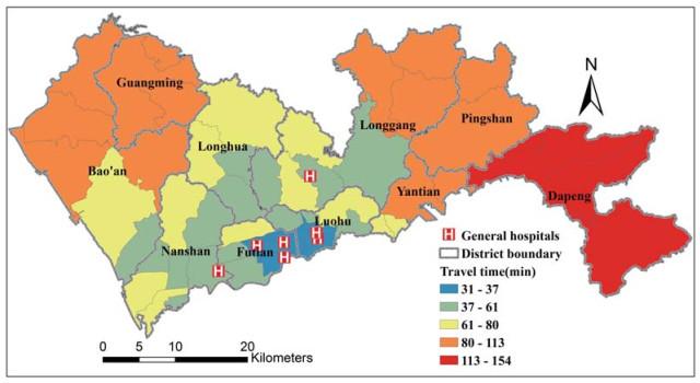The proportion of travel by public transportation in motorized travel is 56 percent in 2014 in Shenzhen^[18]. The synthesized measure of travel time is calculated as the weighted mean of travel time by transit and by driving. The weights of public transportation and driving are 0.56 and 0.44 respectively, determined by the proportion of travel by the two modes. The distribution of average travel time from subdistricts to tertiary hospitals is shown in Figure 4. As a result of the concentrated distribution of existing tertiary hospitals, the distribution of average travel time to tertiary hospitals shows a similar concentrated pattern. The subdistricts near tertiary hospitals have shorter travel time to hospitals.

Figure 4 Average travel time from each subdistrict to existing tertiary hospitals

Full size|PPT slide

3.4 Solution Algorithm

The traditional

p

-median model is a NP-complete problem which is difficult and highly costly to solve^[2]. The gravity

p

-median is more complicated, thus a heuristic algorithm is needed. Previous studies have focused on several heuristic algorithms, including the steepest descent algorithm, the tabu search algorithm and the simulated annealing algorithm^{[6, 7, 19]}. Following the suggestion by Drezner, et al.^[6], this study chooses the steepest descent algorithm due to its relative advantage in operability and solution efficiency.

The steepest descent algorithm was first proposed by Teitz and Bart^[20] for the solution of the traditional

p

-median problem, and thus is also called Teitz-Bart algorithm. Drezner, et al.^[6] improved it to solve the gravity

p

-median model. In this study, it is further adjusted to solve the proposed modified gravity

p

-median model. Denoting the set of demand nodes as

N

, the set of all candidate facility locations as

A P

, and the set of selected facility locations as

P

, the modified steepest descent algorithm can be operated by the following steps:

Step 1 The initial operation. Randomly select

p

candidate facility locations from the set

A P

, based on which the set of selected facility locations

P

is constructed. Then calculate the total travel distance of MGPM according to formula (10), and denote it as

d i s t a n c e (P)

Step 2 For each candidate facility location

k ⋂ P

, execute the following operations: successively replace

k

by each location

j ⋂ A P - P

, and each iteration obtains a new set of selected facility locations denoted as

P_{j}

; calculate the probability of each facility location being selected by formula (9), and sum up the total probability for each demand node

i

, denoted by

t p r o b (i)

; if

t p r o b (i)

= 0, which means that demand node

i

is inaccessible to any facility within the catchment area in MGPM, reassign an infinite value (in practice it is set as 999999) to

t p r o b (i)

; by doing so, a solution that results in a completely inaccessible demand node is considered infeasible.

Step 3 for each iteration of Step 2: Calculate the total travel distance, and find the alternative location that generates the minimum total travel distance, and denote this minimum total travel distance as distance(

P_{j}

); if

d i s t a n c e (P_{j}) < d i s t a n c e (P)

, replace location

j

k

, and update the set of selected facility locations

P

, otherwise no operation is executed.

Step 4 if the total number of iterations of Steps 2 and 3 does not reach the maximum iteration times

T

(set as 20 times in this study), continue with the next iteration; otherwise, terminate the algorithm, and the current set of selected facility locations

P

and the corresponding total travel distance

d i s t a n c e (P)

are the optimal solution of MGPM. The above solution algorithm is implemented by using Matlab (www.mathworks.com) in this study.

3.5 Settings of Empirical Study

The demand nodes are set as the subdistricts. There are 55 demand nodes in total. The candidate facility locations are also set as the subdistricts, thereby the optimized facility locations can be directly linked to corresponding administrative units, which provides convenience for the implementation of the results. In another word, the optimal locations of tertiary hospitals are determined among the subdistricts.

In addition, there are several key parameters need to be determined: The number of allocated facilities

p

, the distance threshold

r

, the attraction of candidate facility locations, and the distance-decay parameter

β

. As for the number of allocated facilities

p

, this study uses the number of actual tertiary hospitals in Shenzhen (

p = 7

) for the convenience of comparing the optimized solutions with the actual situation. The distance threshold is determined based on the average travel time from subdistricts to existing tertiary hospitals (68 min). Two different distance thresholds are considered in this study: 68 min and 105 min (1.5 times of 68 min). Regarding the attraction of candidate facility locations and the distance-decay parameter

β

, we test different scenarios to measure the sensitivity of optimization results on these two parameters.

One superiority of the gravity

p

-median model is that the attractions of candidate facility locations can be variant. In the baseline scenario, the attractions of candidate facility locations are considered higher in central areas and lower in periphery areas in Shenzhen. To observe a clearer difference, the attraction of candidate locations in Luohu, Futian and Nanshan are set as 3 times of locations in other districts. An additional scenario with unitary attraction is set up for a comparison with the baseline scenario, thus examining the difference between the gravity

p

-median model and the

p

-median model.

Due to the lack of adequate information about the exact value of the distance-decay parameter

β

, any single value of

β

is more or less arbitrary. Therefore,

β

should take various values by conducting a sensitivity analysis. Since 1 to 2 is the most common range of

β

in relevant empirical studies, two scenarios where

β

is 1 and 2 respectively are both employed in this study, to investigate the sensitivity of optimization results on

β

To make a brief summary, three parts of empirical analyses are designed in this study. In the first part, two scenarios with unitary and variant attraction of candidate facility locations are calculated for GPM, and are compared with the results of PM, to examine whether the difference in attraction has impact on the results of two models. In the second part, two scenarios with different distance-decay parameters for GPM are calculated and compared, to investigate the impact of distance-decay parameter on optimization results. The third part is designed to compare MGPM with GPM. The two models have the same distance-decay parameter, but MGPM has a distance threshold while GPM does not. Furthermore, all the above scenarios are compared with the distribution of existing tertiary hospitals in Shenzhen.

4 Results

4.1 Examining the Difference Between GPM and PM

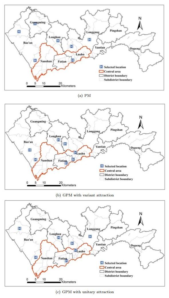
We first compare three scenarios: GPM with unitary attraction of candidate facility locations, GPM with variant attraction, and PM. The distribution of selected facilities by PM is the most dispersed, with only one facility in the central area (Figure 5(a)). The distribution of selected facilities by GPM with variant attraction is the most concentrated in the central area (Figure 5(b)). The distribution of selected facilities by GPM with unitary attraction (Figure 5(c)) is quite similar to the solution of PM, with two facilities located in the central area.

Figure 5 Optimal facility locations by (a) PM, (b) GPM with variant attraction and (c) GPM with unitary attraction

Full size|PPT slide

There are two aspects where GPM is different from PM: The gravity rule of facility selection and variable attraction of candidate facility locations. The results show significant difference between the solutions of GPM with variant attraction and PM, while the solution of GPM with unitary attraction (where only the gravity rule is included) is relatively similar with PM. It can be concluded that the variable attraction of GPM has a dominating impact on the difference between the solutions of GPM and PM, while the gravity rule of facility selection itself has little impact, which has not been revealed by existing studies.

The average travel time is also calculated for each scenario (Table 1). The facility selection rules are different between GPM and PM. The average travel time of GPM is termed as gravity-rule travel time, and the average travel time of PM is termed as nearest-rule travel time. Both gravity-rule and nearest-rule average travel time are calculated for existing tertiary hospitals.

Table 1 Average travel time of PM and GPM (unit: min)

Type	Actual situation	PM	GPM (variant attraction)	GPM (unitary attraction)
Nearest-rule	52.4	35.8	–	–
Gravity-rule	68.3	–	60.5	60.4

As shown in Table 1, the solution of PM reduces the nearest-rule average travel time to a great extent compared with the existing allocation, indicating that PM can significantly minimize the average/total travel cost. The solutions of GPM also result in a smaller gravity-rule average travel time than the existing allocation, but to a limited extent. However, it is no necessarily to conclude that PM is more efficient than GPM. The improvements made by GPM are aimed to model the facility selection behavior more realistically, rather than to pursue a smaller travel cost than PM. In fact, the optimal total travel time obtain by PM is theoretically the smallest, thus other models are impossible to surpass PM in this aspect^[6].

4.2 Impacts of Distance-Decay Parameter on GPM Solution

In this part, two scenarios with different distance-decay parameters (

β

=1 and

β

=2) for GPM are calculated and compared. As shown in Figure 6, the distance-decay parameter does have a significant impact on the solution of GPM. In the scenario with a larger distance-decay parameter, the distribution of selected facilities is more dispersed. The reason is, when the distance-decay parameter is larger, demanders tend to have a larger probability of selecting nearer facilities, thus the optimal facilities tend to be located closer to the demanders. Moreover, a larger distance-decay parameter tends to result in a smaller gravity-rule average travel time (Table 2).

Figure 6 Optimal facility locations by GPM (β=2)

Full size|PPT slide

Table 2 Average travel time of GPM (unit: min)

Actual situation	GPM ( $β$ =1)	GPM ( $β$ =2)
68.3	60.5	53.7

4.3 Impacts of Distance Threshold on MGPM Solution

In this part, two scenarios for MGPM with different catchment areas (

r

=68 or 105 min) are compared to investigate the impacts of distance threshold on the solution of MGPM. We also compare the two scenarios of MGPM with GPM that does not have a distance threshold. For the convenience of comparison, the distance-decay parameter is set as the same (

β

=1) for both MGPM and GPM. Since the distance threshold is the only difference between MGPM and GPM, the impact of distance-decay parameter on the solution of GPM should be analogous for MGPM. Therefore, there is no need to further analyze the impact of distance-decay parameter on the solution of MGPM.

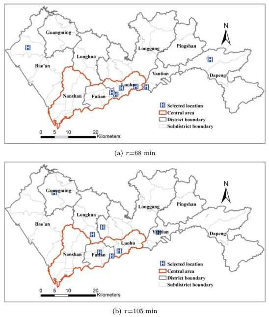
In the MGPM (

r

=68 min) scenario, the distribution of selected facilities (Figure 7(a)) is quite different from the scenario without distance threshold (i.e., GPM solution) (Figure 5(b)). In the MGPM (

r

=68 min) scenario, two facilities are located far away from the central area, one in Bao'an, and one in Dapeng. This is different from all aforementioned scenarios of three models, which suggests that the distance threshold of 68 min has a significant impact on the solution of MGPM, and can promote the spatial equity of tertiary hospital services between periphery and central areas. A larger distance threshold of 105 min (Figure 7(b)), however, is proven to be of much less impact on the solution of MGPM.

Figure 7 Optimal facility locations by PM model when distance threshold is (a) 68 min or (b) 105 min

Full size|PPT slide

The distance threshold also has impacts on the gravity-rule average travel time of MGPM solutions. As shown in Table 3, both scenarios of MGPM result in a smaller gravity-rule average travel time than the actual situation. But the situation becomes different when compared with GPM. The gravity-rule average travel time of MGPM (

r

=68 min) scenario is smaller than GPM, while the average travel time of MGPM (

r

=105 min) scenario is larger than GPM.

Table 3 Average travel time of GPM and MGPM (unit: min)

Actual situation	GPM ( $β$ =1)	MGPM ( $β$ =1, $r$ =68)	MGPM ( $β$ =1, $r$ =105)
68.3	60.5	56.3	62.9

5 Conclusions

The gravity

p

-median model is an important improvement to the widely-used

p

-median model. However, there is still a debate on its validity in empirical applications. Previous studies even doubt the significance of the gravity

p

-median model. This study has re-examined the difference between the gravity

p

-median model with the

p

-median model, by decomposing the difference between the two models into gravity rule and variant attraction. This study has also modified the gravity

p

-median model by incorporating a distance threshold. Using a case study of tertiary hospitals in Shenzhen, China, the proposed modified gravity

p

-median model, the gravity

p

-median model, and the traditional

p

-median model have been compared. Based on the comparisons, the empirical validity and performance of both the gravity

p

-median model and the proposed model have been examined. Several conclusions have been drawn.

First, the optimization result of the gravity

p

-median model shows significant difference from the traditional

p

-median model, and the main impact factor is the variable attraction of candidate facility locations rather than the gravity rule of facility selection. This supports the validity of the gravity

p

-median model, and also reveals the mechanism considering what components of the gravity

p

-median model will lead to different results with the

p

-median model. We conclude that only when the attractions of candidate facility locations are variable, the gravity

p

-median model will lead to different results compared to the

p

-median model. This mechanism has not been revealed by existing studies.

Second, the

p

-median model can reduce the average travel time to a great extent, while the gravity

p

-median model results in limited reduction in average travel time. But it should not be concluded that the gravity

p

-median model is less efficient than the

p

-median model, because the main objective of the gravity

p

-median model is to establish a gravity-style assumption of facility selection behavior. The two models should be applied to match different situations and different facilities.

Third, the solution of the gravity

p

-median model is sensible to the distance-decay parameter. A larger distance-decay parameter tends to result in a more dispersed distribution of selected facilities, and a smaller average travel time. These impacts should be analogous for the proposed modified gravity

p

-median model.

Fourth, the distance threshold of 68 min has impacts on the solution of the modified gravity

p

-median model, and can promote the spatial equity of tertiary hospital services between periphery and central areas, while the impact a larger distance threshold of 105 min is quite limited. A sensitivity analysis on the distance threshold is necessary in cases where adequate information is lacked.

The empirical results of this study can also contribute to the knowledge-based decision-making of tertiary hospitals planning in Shenzhen. The proposed method can be applied in relevant studies of other types of public facilities or in other areas.

References

Publishing order | Descend order by publishing year | Descend order by cited within

1	Drezner Z, Hamacher H W. Facility location: Applications and theory. New York: Springer, 2002. Cited in this article [1]

2	Owen S H, Daskin M S. Strategic facility location: A review. European Journal of Operational Research, 1998, 111, 423- 447. https://doi.org/10.1016/S0377-2217(98)00186-6 Cited in this article [4]

3	Fang L, Li H. Pluralistic efficiency-equity tradeoffs in locating public services. Journal of Systems Science and Information, 2014, 2 (2): 130- 143. https://doi.org/10.1515/JSSI-2014-0130

4	Hakimi S L. Optimum locations of switching centers and the absolute centers and medians of a graph. Operations Research, 1964, 12, 450- 459. https://doi.org/10.1287/opre.12.3.450 Cited in this article [1]

5	White J A, Case K E. On covering problems and the central facilities location problem. Geographical Analysis, 1974, 6, 281- 294. Cited in this article [1]

6	Drezner T, Drezner Z. The gravity $p$ -median model. European Journal of Operational Research, 2007, 179, 1239- 1251. https://doi.org/10.1016/j.ejor.2005.04.054 Cited in this article [11]

7	Carling K, Han M, Hȧkansson J, et al. Testing the gravity $p$ -median model empirically. Operations Research Perspectives, 2015, 2, 124- 132. https://doi.org/10.1016/j.orp.2015.06.002 Cited in this article [4]

8	Zhu J. Non-linear integer programming model and algorithms for connected $p$ -facility location problem. Journal of Systems Science and Information, 2014, 2 (5): 451- 460. https://doi.org/10.1515/JSSI-2014-0451 Cited in this article [1]

9	Luo W, Wang F. Measures of spatial accessibility to health care in a GIS environment: Synthesis and a case study in the Chicago region. Environment and Planning B: Planning and Design, 2003, 30, 865- 884. https://doi.org/10.1068/b29120 Cited in this article [1]

10	McGrail M R. Spatial accessibility of primary health care utilising the two step floating catchment area method: An assessment of recent improvements. International Journal of Health Geographics, 2012, 11, 50. https://doi.org/10.1186/1476-072X-11-50 Cited in this article [1]

11	Fortney J, Rost K, Warren J. Comparing alternative methods of measuring geographic access to health services. Health Services and Outcomes Research Methodology, 2000, 1, 173- 184. https://doi.org/10.1023/A:1012545106828 Cited in this article [1]

12	Haynes R, Jones A P, Sauerzapf V, et al. Validation of travel times to hospital estimated by GIS. International Journal of Health Geographics, 2005, 5, 40. Cited in this article [1]

Ni J, Wang J, Rui Y, et al. An enhanced variable two-step floating catchment area method for measuring spatial accessibility to residential care facilities in Nanjing. International Journal of Environment Research and Public Health, 2015, 12, 14490- 14504.

https://doi.org/10.3390/ijerph121114490

Cited in this article [2]

14	Jia T, Tao H, Qin K, et al. Selecting the optimal healthcare centers with a modified $P$ -median model: A visual analytic perspective. International Journal of Health Geographics, 2014, 13, 42. https://doi.org/10.1186/1476-072X-13-42 Cited in this article [2]

15	Wang F, Xu Y. Estimating O-D travel time matrix by Google Maps API: Implementation, advantages, and implications. Annals of GIS, 2011, 17, 199- 209. https://doi.org/10.1080/19475683.2011.625977 Cited in this article [3]

16	Cheng G, Zeng X, Duan L, et al. Spatial difference analysis for accessibility to high level hospitals based on travel time in Shenzhen, China. Habitat International, 2016, 53, 485- 494. https://doi.org/10.1016/j.habitatint.2015.12.023

17	Gu W, Wang X, McGregor S E. Optimization of preventive health care facility locations. International Journal of Health Geographics, 2010, 9, 17. https://doi.org/10.1186/1476-072X-9-17 Cited in this article [1]

18	Transport Commission of Shenzhen. Index of public transportation services in 2014 in Shenzhen. Available online: http://www.sztb.gov.cn/jtzx/gzdt/gjdt_80994/201503/t20150323_5264499.htm, Accessed on Jan. 25, 2017. Cited in this article [1]

19	Mladenović N, Brimberg J, Hansen P, et al. The $p$ -median problem: A survey of metaheuristic approaches. European Journal of Operational Research, 2007, 179, 927- 939. https://doi.org/10.1016/j.ejor.2005.05.034 Cited in this article [1]

20	Teitz M B, Bart P. Heuristic methods for estimating the generalized vertex median of a weighted graph. Operations Research, 1968, 16, 955- 961. https://doi.org/10.1287/opre.16.5.955 Cited in this article [1]

PDF(811 KB)

295

Accesses

Citation

Detail

Sections

Recommended

Abstract
Key words
Cite this article
1 Introduction
2 Methodology
2.1 The $p$ -Median Model
2.2 The Gravity $p$ -Median Model
2.3 The Modified Gravity $p$ -Median Model
Figure 1 Schematic diagram of three models
3 Data and Calculation
3.1 Study Area
Figure 2 Administrative divisions in Shenzhen
3.2 Data Source of Population and Tertiary Hospitals
Figure 3 Distribution of population and tertiary hospitals in Shenzhen
3.3 Travel Time Estimation
Figure 4 Average travel time from each subdistrict to existing tertiary hospitals
3.4 Solution Algorithm
3.5 Settings of Empirical Study
4 Results
4.1 Examining the Difference Between GPM and PM
Figure 5 Optimal facility locations by (a) PM, (b) GPM with variant attraction and (c) GPM with unitary attraction
Table 1 Average travel time of PM and GPM (unit: min)
4.2 Impacts of Distance-Decay Parameter on GPM Solution
Figure 6 Optimal facility locations by GPM (β=2)
Table 2 Average travel time of GPM (unit: min)
4.3 Impacts of Distance Threshold on MGPM Solution
Figure 7 Optimal facility locations by PM model when distance threshold is (a) 68 min or (b) 105 min
Table 3 Average travel time of GPM and MGPM (unit: min)
5 Conclusions
References

Received	Accepted	Published
2017-05-28	2017-12-07	2018-10-25
Issue Date
2018-10-25

Please choose a citation manager

Content to export

Abstract

Key words

Cite this article

1 Introduction

2 Methodology

2.1 The $p$ -Median Model

2.2 The Gravity $p$ -Median Model

2.3 The Modified Gravity $p$ -Median Model

Figure 1 Schematic diagram of three models

3 Data and Calculation

3.1 Study Area

Figure 2 Administrative divisions in Shenzhen

3.2 Data Source of Population and Tertiary Hospitals

Figure 3 Distribution of population and tertiary hospitals in Shenzhen

3.3 Travel Time Estimation

Figure 4 Average travel time from each subdistrict to existing tertiary hospitals

3.4 Solution Algorithm

3.5 Settings of Empirical Study

4 Results

4.1 Examining the Difference Between GPM and PM

Figure 5 Optimal facility locations by (a) PM, (b) GPM with variant attraction and (c) GPM with unitary attraction

Table 1 Average travel time of PM and GPM (unit: min)

4.2 Impacts of Distance-Decay Parameter on GPM Solution

Figure 6 Optimal facility locations by GPM (β=2)

Table 2 Average travel time of GPM (unit: min)

4.3 Impacts of Distance Threshold on MGPM Solution

Figure 7 Optimal facility locations by PM model when distance threshold is (a) 68 min or (b) 105 min

Table 3 Average travel time of GPM and MGPM (unit: min)

5 Conclusions

{{custom_sec.title}}

{{custom_sec.title}}

References

{{custom_fnGroup.title_en}}

Footnotes

Share

模态框（Modal）标题

Please choose a citation manager

Content to export

Abstract

Key words

Cite this article

1 Introduction

2 Methodology

2.1 The p-Median Model

2.2 The Gravity p-Median Model

2.3 The Modified Gravity p-Median Model

Figure 1 Schematic diagram of three models

3 Data and Calculation

3.1 Study Area

Figure 2 Administrative divisions in Shenzhen

3.2 Data Source of Population and Tertiary Hospitals

Figure 3 Distribution of population and tertiary hospitals in Shenzhen

3.3 Travel Time Estimation

Figure 4 Average travel time from each subdistrict to existing tertiary hospitals

3.4 Solution Algorithm

3.5 Settings of Empirical Study

4 Results

4.1 Examining the Difference Between GPM and PM

Figure 5 Optimal facility locations by (a) PM, (b) GPM with variant attraction and (c) GPM with unitary attraction

Table 1 Average travel time of PM and GPM (unit: min)

4.2 Impacts of Distance-Decay Parameter on GPM Solution

Figure 6 Optimal facility locations by GPM (β=2)

Table 2 Average travel time of GPM (unit: min)

4.3 Impacts of Distance Threshold on MGPM Solution

Figure 7 Optimal facility locations by PM model when distance threshold is (a) 68 min or (b) 105 min

Table 3 Average travel time of GPM and MGPM (unit: min)

5 Conclusions

{{custom_sec.title}}

{{custom_sec.title}}

References

{{custom_fnGroup.title_en}}

Footnotes

2.1 The $p$ -Median Model

2.2 The Gravity $p$ -Median Model

2.3 The Modified Gravity $p$ -Median Model