A Model of Aircraft Support Concept Evaluation Based on DEA and PCA

Bin LIN; Dong SONG; Zhiyue LIU

doi:10.21078/JSSI-2018-563-14

PDF(310 KB)

Journal of Systems Science and Information ›› 2018, Vol. 6 ›› Issue (6) : 563-576. DOI: 10.21078/JSSI-2018-563-14

A Model of Aircraft Support Concept Evaluation Based on DEA and PCA

Author information +

History +

Abstract

With the vigorous development of equipment manufacturing industry in China, higher requirements to the equipment supportability are put forward. How to evaluate the supportability of equipments (especially the aviation equipment-aircraft) objectively and correctly is the problem to be solved in the development of aviation equipments construction, demonstration and battle application. Aimed at the needs of the supportability analysis of complex equipment systems-aircraft, a model of aircraft support concept evaluation based on DEA (data envelopment analysis) and PCA (principal component analysis) is proposed. The model is used to evaluate a certain aircraft support concept. The process and the results of evaluation show that proposed model is feasible and effective. The model is suitable for advanced aircraft support concept evaluation. The feasibility and effectiveness of the proposed model is verified by the analysis of the evaluation results. This method is applicable to the evaluation of aircraft support concepts.

Key words

aircraft supportability / data envelopment analysis(DEA) / concept evaluation

Cite this article

EndNote

Ris (Procite)

Bibtex

Download Citations

Bin LIN , Dong SONG , Zhiyue LIU. A Model of Aircraft Support Concept Evaluation Based on DEA and PCA. Journal of Systems Science and Information, 2018, 6(6): 563-576 https://doi.org/10.21078/JSSI-2018-563-14

1 Introduction

With the push of the high-tech and the need of the force, many new technologies have been used in military equipment. The complexity and the integration of the weapon increase exponentially. The problem of equipment supportability raises more and more attention. As a kind of the complex equipment system, the support requirements of the aircraft are very complex. The supportability analysis and evaluation during the whole life cycle can effectively enhance the supportability. Thereby it can improve greatly the efficiency of the aircraft.

The main function of the aircraft comprehensive support is to meet the wartime and peacetime support requirements of the aircraft with the affordable cost of life cycle. The purpose of aircraft comprehensive support is to keep the combat readiness integrity. Considering the problems of supportability during the design comprehensively can improve security characteristics and can determine the best support requirements and can give reasonable acquisition of support resources to provide the necessary protection for users with the lowest cost. Analysis and evaluation with the qualitative and quantitative requirements are generally needed to verify whether the purpose is achieved.

Now the foreign researches on supportability are primary based on the establishment of the universal criteria and indicators, but lack of separate study on aircraft^[1-4]. The domestic relative researches started late^[5]. Some research institutes such as data center of the Center of Analysis the Fifth Research of MII, Beijing University of Aeronautics and Astronautics, National University of Defense Technology, had related researches on supportability modeling and simulation^{[6, 7]}. However, many of the simulation work are not deep enough. There are many contents worthy of study and discussion. First, targeted researches on aircraft are limited. There aren't any universal and complete criterions for the choice of indicators and the design of the concepts^[8-10]. Secondly, most evaluation of the concepts that is qualitative analysis^{[11, 12]}, so it can't perform the concepts quantitatively.

In this paper, the theory and models of DEA are studied and a model of aircraft support concept evaluation based on DEA and PCA is proposed. The model is used to evaluate the certain aircraft support concept. The process and the results of evaluation show that proposed model is feasible and effective. The model is suitable for advanced aircraft support concept evaluation.

2 Theory and Model Analysis of DEA

Data envelopment analysis (DEA) was proposed by famous aspects of operations research, Charnes, Cooper and Rhodes^[13]. It's a new efficiency evaluation method based on the concept of relative efficiency. Mathematical programming model is used to compare the relative efficiency of Decision making units (DMU) and evaluate DMU. Each decision unit has the same input and output in the same case. Through comprehensive analysis of the input and output data, the comprehensive efficiency indicator can be computed to compare DMUs. The indicator determines the effectiveness (i.e., the highest relative efficiency) of a DMU and points out the causes and degree of other DMUs which are not effective. DMU can also determine whether the size of the investment is appropriate and can show the correct direction and scale of DMU investment (i.e., expanding or reducing the investment and the number of changes)^[14].

2.1 Basic Theory of DEA

1) Decision Making Unit

An economic system or a production process refers to economic or productive activities. In the activities, a certain amount of production factors are invested and a certain amount of products are produced in a range of possibilities^[13]. DMU is an agreement that it can be a school, a hospital, a court, an air force base, a bank or an enterprise. The dominant principle of determining DMU is that each DMU can be viewed as the same entity in terms of its "cost of resources" and "production of the product". In the DEA method, each operating entity which transfers a certain amount of inputs to a certain amount of outputs is known as a DMU. All DMUs in the same evaluation object have the same type of input and output, and the difference is only in quantity.

2) Production possibility set and extended model

The input vector and the output vector of a DMU is

X = {(x_{1}, x_{2}, \dots, x_{m})}^{T}

and

Y = {(y_{1}, y_{2}, \dots, y_{s})}^{T} .

(X_{j}, Y_{j})

j = 1, 2, \dots, n

, which represent the entire production activity of the DMU. In particular, observations on these vectors can show which DMUs are relatively effective^{[15, 16]}.

The reference set

T^{'}

is:

\begin{array}{rcl} T^{'} = {(X_{j}, Y_{j}) | j = 1, 2, \dots, n}, \end{array}

(1)

\begin{array}{rcl} T = {(X, Y) | \sum_{j = 1}^{n} x_{j} λ_{j} \leq X, \sum_{j = 1}^{n} y_{j} λ_{j} \leq Y, λ_{j} \geq 0}, \end{array}

(2)

where

m

is the number of inputs,

s

is the number of output and

n

is the number of DMU,

T

is the production possibility set.

2.2 C $^{2}$ R

There are

n

DMUs. Each of DMU has

m

kinds of inputs (i.e., the resource consumption of a DMU), and

s

kinds of outputs (i.e., some indicators of "effectiveness"). An illustration is shown in Figure 1.

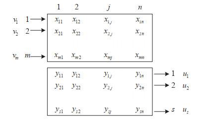
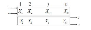
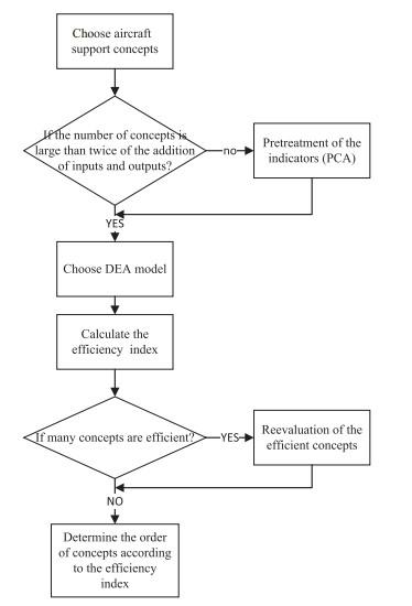
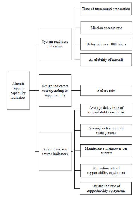
Figure 1 The inputs and the outputs of DEA

Full size|PPT slide

Where,

x_{i j}

is the amount of the

i

th input of the

j

th DMU;

y_{r j}

is the amount of the

r

th output of the

j

th DMU;

v_{i}

is weight of the

i

th input;

u_{r}

is weight of the

r

th output,

x_{i j} > 0, y_{r j} > 0, v_{i} \geq 0, u_{r} \geq 0, i = 1, 2, \dots, m; r = 1, 2, \dots, s; j = 1, 2, \dots, n

x_{i j}

and

y_{r j}

is known from the historical data or forecast. The vector form of the input and output is shown in Figure 2.

Figure 2 Vectors of the inputs and outputs

Full size|PPT slide

The efficiency evaluation index of EMU

_{j}

based on weight vector

v \in E^{m}

and

u \in E^{s}

is:

\begin{array}{rcl} h_{j} = \frac{u^{T} Y_{j}}{v^{T} X_{j}}, j = 1, 2, \dots, n, \end{array}

(3)

The

h_{j}

is efficiency evaluation index. It represents the ratio of the investment

v^{T} X_{j}

and production

u^{T} Y_{j}

. When

X_{0} = X_{j_{0}}, Y_{0} = Y_{j_{0}}, 1 \leq j_{0} \leq n

, the method refers to

h_{j_{0}}

as objective. The efficiency evaluation index of all DMU

_{s}

including DMU

_{j}

is a constraint. The fractional programming problem (C

^{2}

R model) can be get using Equation (4)^[17].

\begin{array}{rcl} {(C^{2} R)}^{I} {\begin{cases} max \frac{u^{T} Y_{0}}{v^{T} X_{0}} = V^{I} P, \\ \frac{u^{T} Y_{j}}{v^{T} X_{j}} \leq 1, j = 1, 2, \dots, n, \\ u \geq 0, v \geq 0, \end{cases} \end{array}

(4)

Many improved models were proposed^{[16, 18, 19]}. Charnes and Cooper improved the

D_{C^{2} R}^{I}

model. They proposed a new DEA model (

D_{ε}^{I}

) with non-Archimedes infinitely small quantity. The Equation (4) is transferred into Equation (5).

\begin{array}{rcl} {\begin{cases} max \frac{u^{T} Y_{0}}{v^{T} X_{0}}, \\ \frac{u^{T} Y_{J}}{v^{T} X_{J}} \leq 1, j = 1, 2, \dots, n, \\ \frac{v}{v^{T} X_{J}}, \\ \frac{u}{v^{T} X_{J}}, \end{cases} \end{array}

(5)

where

\begin{aligned} \hat{e} = {(1, 1, \dots, 1)}^{T} \in E^{m}, e = {(1, 1, \dots, 1)}^{T} \in E^{s} . \end{aligned}

The dual programming of model is:

\begin{array}{rcl} (D_{ε}^{I}) {\begin{cases} min [θ - ε ({\hat{e}}^{T} S^{-} + e^{T} S^{+})], \\ \sum_{j = 1}^{n} X_{j} λ_{j} + S^{-} = θ X_{0}, \\ \sum_{j = 1}^{n} Y_{j} λ_{j} - S^{+} = Y_{0}, \\ λ_{j} \geq 0, j = 1, 2, \dots, n, \\ S^{-} \geq 0, S^{+} \geq 0. \end{cases} \end{array}

(6)

Where

S^{-} = (S_{1}^{-}, S_{2}^{-}, \dots, S_{m}^{-})

is the slack variable of

m

inputs.

λ = (λ_{1}, λ_{2}, \dots, λ_{n})

is the combination coefficient of

n

DMU

_{s}

e_{1}^{T} = {(1, 1, \dots, 1)}_{1 \times m}

e_{2}^{T} = {(1, 1, \dots, 1)}_{1 \times s}

ε

is an infinitely small quantity.

ε = 10^{- 6}

is taken generally.

Optimization solution

θ^{0}

of C

^{2}

R model (

D_{ε}^{I}

) is calculated.

θ^{0}

is the relative efficiency index of

j_{0}

1) If

θ^{0} < 1

, then support concept DMU

_{j_{0}}

is non-efficient for DEA.

2) If

θ^{0} = 1, {\hat{e}}^{T} S^{- 0} + S^{+ 0} > 0

, then support concept DMU

_{j_{0}}

is weak-efficient for DEA.

3) If

θ^{0} = 1, {\hat{e}}^{T} S^{- 0} + S^{+ 0} = 0

, then support concept DMU

_{j_{0}}

is efficient for DEA.

In this paper, C

^{2}

R model(

D_{ε}^{I}

) is chosen to calculate the relative efficiency index.

3 Evaluation of Aircraft Support Concept Based on DEA

3.1 Evaluation Process of DEA

The basic analysis of the DEA evaluation model is: 1) Calculate relative efficiency index of the support concept; 2) Evaluate the efficiency of the concept. Concept is judged whether located on the "frontier" of the possibility set. The "frontier" is formed by the efficient concepts in possibility set^[20].

The flow of DEA application is as follow: 1) Determine the purpose of the evaluation; 2) Choose DMUs and build the system of inputs and outputs; 3) Collect and organize the data; 4) Choose the proper DEA model and calculate; 5) Analyze the results and give suggestions. The chart of flow is shown in Figure 3.

Figure 3 Flow of aircraft support concept evaluation based on DEA method

Full size|PPT slide

3.2 Determination of Input and Output Indicators

Comprehensive parameters and design parameters related to supportability and system/source of supportability are used to establish the supportability evaluation indicators of aircraft. Considering the availability, operability and importance of basic evaluation data, 10 indicators are chosen from the comprehensive indicator system. They are time of turnaround preparation^[21], average delay time of supportability resources, delay rate per 1000 times, failure rate, average delay time for management, maintenance manpower per aircraft, availability of aircraft, mission success rate, satisfaction rate of supportability equipment, utilization rate of supportability equipment. The system is shown in Figure 4.

Figure 4 Indicator System of the supportability evaluation

Full size|PPT slide

Cooper, Seiford and Tone gave selection basis of the traditional DEA for "input" and "output" in book《Data Envelopment Analysis》^{[22, 23]}. The method is as follow: 1) Every input and output of all DMU should be positive; 2) These parts including inputs, outputs, the selection of DMUs, should reflect interest of the analyzers and managers about the related elements; 3) Considering with the principle of the efficiency ratio, the value of the inputs should be small and the value of the outputs should be large; 4) Different inputs and outputs don't required the same unit. Dimension doesn't need to be unified. It can be number of people, size and cost and so on. The indicators chosen are divided into inputs which are smaller and better and outputs which are bigger and better. The results are shown in Table 1.

Table 1 Indicator System of inputs and outputs

Input indicator	Output indicator
X₁ time of turnaround preparation /h	Y₁ availability of aircraft /%
X₂ average delay time for management /h	Y₂ mission success rate /%
X₃ delay rate per 1000 time/%	Y₃ satisfaction rate of supportability equipment /%
X₄ failure rate/%	Y₄ utilization rate of supportability equipment /%
X₅ average delay time for management /h
X₆ maintenance manpower per aircraft(MM/AC)

3.3 Indicator Pretreatment

In the research of aircraft supportability, many indicators are set and the data are collected for comprehensive performance of the system. A large amount of the indicators not only increase the complexity of the analysis, but also neglect the information overlapping of the indicators.

Principal component analysis (PCA) was proposed by Karl and Pearson in 1901. It was applied to non-random variables. In 1933, Hotelling extend this concept to random vectors. This multivariate statistical analysis method is used to reduce dimensions, which transfer multiple indicators into a few ones. Its basic principle is turning a set of correlate variables into another set of uncorrelated variables. These new variables are arranged in descending order of variance. The total variance remains in the mathematical transformation. The first variable has the largest variance, which is called first principal component. The second variable has the second largest variance, which is called second principal component. The

k

th variable corresponds to the

k

th principal component. New names can be given to the principal components according to the professional knowledge and the unique meaning of principal components, in order to explain the new variables^{[24, 25]}. The steps of PCA applied to indicator pretreatment are as follows:

Step 1 Normalization of original indicators

The data matrix is denoted as

X = {(X_{i j})}_{n \times p}, i = 1, 2, \dots, n; j = 1, 2, \dots, p

, where

n

is the number of the samples and

p

is the number of the indicators. The

x_{i j}

j

th indicator of the

i

th example.

\begin{array}{rcl} X = [\begin{array}{c} x_{11} & x_{12} & \dots & x_{1 p} \\ x_{21} & x_{22} & \dots & x_{2 p} \\ ⋮ & ⋮ & ⋱ & ⋮ \\ x_{n 1} & x_{n 2} & \dots & x_{n p} \end{array}] . \end{array}

(7)

The data are normalized by

Z

-score method.

Z

is the normalized matrix.

\begin{array}{rcl} Z_{i j} = \frac{x_{i j} - x_{j}}{s_{j}}, i = 1, 2, \dots, n; j = 1, 2, \dots, p, \end{array}

(8)

where

\begin{aligned} \bar{x_{j}} = \frac{\sum_{i = 1}^{n} x_{i j}}{n}, s_{j}^{2} = \frac{\sum_{i = 1}^{n} {(x_{i j} - \bar{x_{j}})}^{2}}{n - 1}, \end{aligned}

\begin{array}{rcl} Z = [\begin{array}{c} z_{1}^{T} \\ z_{2}^{T} \\ ⋮ \\ z_{n}^{T} \end{array}] = [\begin{array}{c} z_{11} & z_{12} & \dots & z_{1 p} \\ z_{21} & z_{22} & \dots & z_{2 p} \\ ⋮ & ⋮ & ⋱ & ⋮ \\ z_{n 1} & z_{n 2} & \dots & z_{n p} \end{array}] . \end{array}

(9)

Step 2 Calculate the correlation matrix of the normalized matrix

Z

R = {(r_{j k})}_{p \times p}, j = 1, 2, \dots, p; k = 1, 2, \dots, p,

where

r_{j k}

is the correlation coefficient of

j

th indicator and

k

th indicator.

\begin{array}{rcl} r_{j k} = \frac{Z^{T} Z}{n - 1} = \frac{1}{n - 1} \sum_{i = 1}^{n} [(x_{i j} - \bar{x_{j}}) / S_{j}] [((x_{i k} - \bar{x_{k}}) / S_{k})], \end{array}

(10)

i.e.,

\begin{array}{rcl} r_{j k} = \frac{Z^{T} Z}{n - 1} = \frac{1}{n - 1} \sum_{i = 1}^{n} [(x_{i j} - \bar{x_{j}}) / S_{j}] [((x_{i k} - \bar{x_{k}}) / S_{k})], \end{array}

(11)

where

r_{i i} = 1, r_{j k} = r_{k j}; i = 1, 2, \dots, n; j = 1, 2, \dots, p; k = 1, 2, \dots, p

Step 3 Find characteristic value and eigenvectors of the correlation matrix

R

and determine the principal component

p

characteristic value that can be obtained by through the equation

| λ I - R | = 0

, where

λ_{1} \geq λ_{2} \geq \cdot \cdot \cdot \geq λ_{p} \geq 0

. The corresponding eigenvector is

a_{i} = {(a_{1 i}, a_{2 i}, \dots, a_{p i})}^{T}

, where

i = 1, 2, \dots, p

M

principal components which are no less than 1 will be extracted, or determine the

m

through equation

\sum_{j = 1}^{m} λ_{j} / \sum_{j = 1}^{p} λ_{j} \geq 0.85

. The utilization rate of the information can be over 85

%

in this way. Every

λ_{j}

j = 1, 2, \dots, m

matches its unit-eigenvector

α_{j}^{o}

through the equation

R α^{o} = λ_{j} α

Step 4 Calculate the score of principal components The

i

th principal component is:

\begin{array}{rcl} F_{i} = α_{1 i} Z_{1} + α_{2 i} Z_{2} + \dots + α_{p i} Z_{p}, i = 1, 2, \dots, p, \end{array}

(12)

F_{i}

is set as the value of the new evaluation indicator.

4 A Case of a Certain Aircraft Support Concept Evaluation (Case Study)

In practical engineering, there are a few number of the support concepts in usage stage. The efficient concepts will be more if the number of concepts is less than two times of the addition of input and output indicators. It results in the bad performance of distinguishing the concepts. PCA is used in the pretreatment of indicators to solve this problem. News indicators which maintain the main information of the original ones, are given as the linear combination of the original relative ones. The indicators are pretreated in the following process:

4.1 PCA of the Input and Output Indicators

The coefficient matrix of principal components COEFF, eigenvectors of correlation coefficient matrix of the sample, Hotelling T2-statistic observed, contribution rate, accumulative contribution rate etc. are calculated. The results are shown in Table 2 and Table 3.

Table 2 Total variance decomposition of input indicators

principal component factors	correlation matrix
principal component factors	eigenvalue	variance contribution rate %	Cumulative contribution rate %	Eigenvector 1
X₁	4.9578	82.6297	82.6297	0.4429
X₂	0.9292	15.4861	98.1158	0.2059
X₃	0.0841	1.4009	99.5167	0.4450
X₄	0.0290	0.4833	100	0.4398
X₅	0	0	100	0.4240
X₆	0	0	100	0.4361

Table 3 Total variance decomposition of output indicators

principal component factors	correlation matrix
principal component factors	eigenvalue	variance contribution rate %	Cumulative contribution rate %	Eigenvector 1
Y₁	3.9629	99.0723	99.0723	0.5018
Y₂	0.0249	0.6237	99.696	0.5004
Y₃	0.0111	0.2784	99.9744	0.4999
Y₄	0.0010	0.0256	100	0.4979

According to the principle that eignvalue should be no less than 1 or accumulation contribution rate should be higher than a level (e.g., 85

%

X_{1}^{'}

was extracted for input indicators and

Y_{1}^{'}

was extracted for output indicators. The results are shown in Table 4 and Table 5.

Table 4 The principal component extraction result of input indicators

principal component factors	correlation matrix
principal component factors	eigenvalue	variance contribution rate %	Cumulative contribution rate %	Eigenvector 1
X'₁	4.9578	82.6297	82.6297	0.4429

Table 5 The principal component extraction result of output indicators

principal component factors	correlation matrix
principal component factors	eigenvalue	variance contribution rate %	Cumulative contribution rate %	Eigenvector 1
Y'₁	3.9629	99.0723	99.0723	0.5018

4.2 The Principal Composition of the Input and Output Indicators

The principal composition of the input and output indicators were calculated by Equation (12). The results were set as the new indicators. It is the input indicators. It is the output indicators. The results are shown in Table 6 and Table 7.

Table 6 It is the output indicator

indicator	concept
indicator	concept 1	concept 2	concept 3	concept 4	concept 5
X'₁	-1.7237	3.8130	-1.3740	-0.0595	-0.6558

Table 7 Simplified output indicator data

indicator	concept
indicator	concept 1	concept 2	concept 3	concept 4	concept 5
Y'₁	2.0024	-3.0859	1.3256	-0.6372	0.3950

4.3 The Determination of the Final Indicator System

According to the results of new indicator, input and output indicators were calculated. As the values of input and output indicators cannot satisfy the principle of DEA model, i.e.,

x_{j} = (x_{1 j}, x_{2 j}, \dots, x_{m j})^{T} > 0, y_{j} = (y_{1 j}, y_{2 j}, \dots, y_{s j})^{T} > 0,

the indicators were corrected. Linear change with no influence in results was used to these indicators. The negative indicators were changed through Addition transform. The transform formula is:

\begin{array}{rcl} X_{j} = X_{j} + α, Y_{j} = Y_{j} + β, \end{array}

(13)

where

X_{j}, Y_{j}

are the input and output vectors of the

j

th concept;

α

is the non-negative transform of the inputs;

β

is the non-negative transform of the outputs. In this way, all the inputs and outputs can be positive. In the meantime, the frontier of the concepts is shifted without any change of shape, i.e., the effectiveness of concepts is not change. In this paper,

α = 2, β = 3,

final indicators were calculated through Equation (13). Results are shown in Table 8 and Table 9.

Table 8 Simplified input indicator data

indicator	concept
indicator	concept 1	concept 2	concept 3	concept 4	concept 5
X'₁	0.2763	5.8130	0.6260	1.9405	1.3442

Table 9 Simplified output indicator data

indicator	concept
indicator	concept 1	concept 2	concept 3	concept 4	concept 5
Y'₁	6.0024	0.9141	5.3256	3.3628	4.3950

4.4 Result and Analysis

In this paper, DEAP version 2.1 was used to implement the DEA model. The relative efficiency of concepts was calculated with the final indicators. The results are shown in Table 10.

Table 10 The order of the support concepts

concept	Relative efficiency value	order
concept 1	1.0000	1
concept 2	0.0072	5
concept 3	0.3916	2
concept 4	0.0798	4
concept 5	0.1505	3

Integration and technical efficiency of 5 concepts was analyzed through VRS model including the index of technological progress, technical efficiency change and scale efficiency change. The results are shown in Table 11.

Table 11 Analysis result of VRS model

concept	total effective value	total effectiveness	pure technical efficiency	effectiveness of Technology	scale efficiency	scale profit
concept 1	1.000	effective	1.000	effective	1.000	invariant
concept 2	0.007	non-effective	0.048	non-effective	0.152	increase
concept 3	0.392	non-effective	0.441	non-effective	0.887	increase
concept 4	0.080	non-effective	0.142	non-effective	0.560	increase
concept 5	0.151	non-effective	0.206	non-effective	0.732	increase
average	0.326		0.367		0.666

The results show that concept 1 is the most effective and the concept 2 is the least. The projection analysis of concepts is shown in Table 12. Input redundancy and output deficiency will be analyzed.

Table 12 The principal component extraction result of output indicators

concept		original value	input redundancy value	output deficiency	target value	strategy
concept 1	output	6.002	0.000	0.000	6.002	Proper production
concept 1	input	0.276	0.000	0.000	0.276	Proper investment
concept 2	output	0.914	0.000	5.088	6.002	output lack
concept 2	input	5.813	-5.537	0.000	0.276	input redundancy
concept 3	output	5.326	0.000	0.677	6.002	output lack
concept 3	input	0.626	-0.350	0.000	0.276	input redundancy
concept 4	output	3.363	0.000	2.640	6.002	output lack
concept 4	input	1.940	-1.664	0.000	0.276	input redundancy
concept 5	output	4.395	0.000	1.607	6.002	output lack
concept 5	input	1.344	-1.068	0.000	0.276	input redundancy

Concept 1:

Pure efficiency = 1.000.

Scale efficiency = 1.000.

The output isn't deficient as the value of output deficiency is 0.

The input isn't redundant as the value of input redundancy is 0.

Concept 2:

Pure efficiency = 0.048.

Scale efficiency = 0.152.

The output is deficient as the original value is 0.914. The value of output deficiency is 5.088 and the target value is 6.002. It means that the output of the sample should be increased to achieve the DEA target value of efficiency.

The input is redundant as the original value is 5.813. The value of input redundancy is

-

5.537 and the target value is 0.276. It means that the input of the sample should be reduced to achieve the DEA target value of efficiency.

Concept 3:

Pure efficiency = 0.441.

Scale efficiency = 0.887.

The output is deficient as the original value is 5.326. The value of output deficiency is 0.677 and the target value is 6.002. It means that the output of the sample should be increased to achieve the DEA target value.

The input is redundant as the original value is 0.626. The value of input redundancy is

-

0.350 and the target value is 0.276. It means that the input of the sample should be reduced to achieve the DEA target value.

Concept4:

Pure efficiency = 0.142.

Scale efficiency = 0.560.

The output is deficient as the original value is 3.363. The value of output deficiency is 2.640 and the target value is 6.002. It means that the output of the sample should be increased to achieve the DEA target value.

The input is redundant as the original value is 1.940. The value of input redundancy is

-

1.664 and the target value is 0.276. It means that the input of the sample should be reduced to achieve the DEA target value.

Concept5:

Pure efficiency = 0.206.

Scale efficiency = 0.732.

The output is deficient as the original value is 4.395. The value of output deficiency is 1.607 and the target value is 6.002. It means that the output of the sample should be increased to achieve the DEA target value.

The input is redundant as the original value is 1.344. The value of input redundancy is

-

1.068 and the target value is 0.276. It means that the input of the sample should be reduced to achieve the DEA target value.

5 Conclusion

A model of aircraft support concept evaluation based on DEA and PCA is proposed in this paper. Index including relative efficiency is used to quantitatively evaluate the concepts. The method is used to evaluate a case of a certain aircraft support concept. The total efficiency, pure technical efficiency and scale efficiency of different concepts is calculated. The process and the results of evaluation show that proposed model is feasible and effective. The model is suitable for advanced aircraft support concept evaluation.

References

Publishing order | Descend order by publishing year | Descend order by cited within

1	U. S. Army Forms Management Officer. Test and evaluation policy. AR73-1, 2004. Cited in this article [1]

2	Michael A B. Logistic test and evaluation in flight test. RTO-AG-300-V20, 2001.

3	Lappin M K. Supportability evaluation prediction process. Reliability and Maintainability Symposium, 1988. Proceedings IEEE, 2002: 102-107.

4	Jones J V. Integrated logistics support handbook. New York: McGraw-Hill, 2006. Cited in this article [1]

5	Wei C C. Research on the implementation of integrated support engineering in the development of military aircraft. Technology Foundation of National Defence, 2006, 1, 32- 34. Cited in this article [1]

6	Xu Z C. Supportability engineering and management for equipment. Beijing: National Defend Industry Press, 2006. Cited in this article [1]

7	Zhang W J, Guo L H. Equipment supportability analysis technology. Beijing: Beijing University of Aeronautics and Astronautics Press, 2012. Cited in this article [1]

8	Guo Y M, Chen D L, Li Z G, et al. Model study on maintenance support ability evaluation of aircraft equipment in wartime. Fire Control & Command Control, 2010, 35 (10): 66- 170. https://doi.org/10.3969/j.issn.1002-0640.2010.10.018 Cited in this article [1]

9	Meng X S, Zhang Y P. A brief discussion on parameter system of aviation equipment supportability. Aeronautic Standardization & Quality, 1997, 3, 40- 44.

10	Ding D H, Lu J. Discussion on the system of reliability, maintainability and supportability parameters. Journal of China Academy of Electronics and Information Technology, 2011, 6 (2): 170- 174. https://doi.org/10.3969/j.issn.1673-5692.2011.02.014 Cited in this article [1]

11	Liu S. DEA-based fuzzy comprehensive evaluation and its applications. Zhejiang: Zhejiang University, 2010. Cited in this article [1]

12	Cao D G, Xu H J, Hu L M, et al. Maintenance support capability evaluation of aeronautical equipment based on RBF neural network. Aeronautical Computing Technique, 2006, 36 (5): 92- 94. https://doi.org/10.3969/j.issn.1671-654X.2006.05.025 Cited in this article [1]

13	Charnes A, Cooper W W, Rhodes E. Measuring the efficiency of decision making units. European Journal of Operational Research, 1978, 6 (2): 429- 444. Cited in this article [2]

14	Wei Q L. Data envelopment analysis (DEA). Chinese Science Bulletin, 2000, 45 (17): 1793- 1808. https://doi.org/10.1360/csb2000-45-17-1793 Cited in this article [1]

15	Banker R D, Charnes A, Cooper W W. Some models for estimating technical and scale inefficiencies in data envelopment analysis. Management Science, 1984, 30 (9): 1078- 1092. https://doi.org/10.1287/mnsc.30.9.1078 Cited in this article [1]

16	Charnes A, Cooper W W, Golany B. Foundations of data envelopment analysis for pareto-koopmans efficient empirical production functions. Journal of Econometrics, 1985, 30 (1): 91- 107. Cited in this article [2]

17	Wang Q W. The further research on DEA-method. Tianjin: Tianjin University, 2008. Cited in this article [1]

18	Charnes A, Cooper W W, Wei Q L. Cone ratio data envelopment analysis and multi-objective programming. Texas: The University of Texas at Austin, 1986. Cited in this article [1]

19	Duan S W, Shen P S. Application of fuzzy comprehensive evaluation and data envelopment analysis in engineering project design. Journal of Hydraulic Engineering, 2004, 35 (5): 116- 121. Cited in this article [1]

20	Chen Y, Li K W, Xu H Y, et al. A DEA-topsis method for multiple criteria decision analysis in emergency management. Journal of Systems Science and Systems Engineering, 2009, 38 (4): 5205- 5211. Cited in this article [1]

21	Wei Y, Kang R, Cheng H L. Calculation method for military aircraft's turnaround time. Journal of Beijing University of Aeronautics and Astronautics, 2008, 34 (12): 1415- 1418. Cited in this article [1]

22	Cooper W W, Seiford L M, Tone K. Data envelopment analysis. Stata Journal, 2010, 10 (2): 267- 280. Cited in this article [1]

23	Li L, Cui J C. Selection of input-output items and data disposal in DEA. Journal of Systems Engineering, 2003, 18 (6): 487- 490. Cited in this article [1]

24	Zhang P. Research on comprehensive evaluation based on principal component analysis. Nanjing: Nanjing University of Science and Technology, 2004. Cited in this article [1]

25	Li Y S, Zeng Z X, et al. Application of principal component analysis in multi index comprehensive evaluation method. Journal of Hebei University of Technology, 1999, 28 (1): 94- 97. Cited in this article [1]

PDF(310 KB)

351

Accesses

Citation

Detail

Sections

Recommended

Abstract
Key words
Cite this article
1 Introduction
2 Theory and Model Analysis of DEA
2.1 Basic Theory of DEA
2.2 C $^{2}$ R
Figure 1 The inputs and the outputs of DEA
Figure 2 Vectors of the inputs and outputs
3 Evaluation of Aircraft Support Concept Based on DEA
3.1 Evaluation Process of DEA
Figure 3 Flow of aircraft support concept evaluation based on DEA method
3.2 Determination of Input and Output Indicators
Figure 4 Indicator System of the supportability evaluation
Table 1 Indicator System of inputs and outputs
3.3 Indicator Pretreatment
4 A Case of a Certain Aircraft Support Concept Evaluation (Case Study)
4.1 PCA of the Input and Output Indicators
Table 2 Total variance decomposition of input indicators
Table 3 Total variance decomposition of output indicators
Table 4 The principal component extraction result of input indicators
Table 5 The principal component extraction result of output indicators
4.2 The Principal Composition of the Input and Output Indicators
Table 6 It is the output indicator
Table 7 Simplified output indicator data
4.3 The Determination of the Final Indicator System
Table 8 Simplified input indicator data
Table 9 Simplified output indicator data
4.4 Result and Analysis
Table 10 The order of the support concepts
Table 11 Analysis result of VRS model
Table 12 The principal component extraction result of output indicators
5 Conclusion
References

Received	Accepted	Published
2017-03-29	2018-03-19	2018-12-25
Issue Date
2018-12-25

模态框（Modal）标题

Please choose a citation manager

Content to export

Abstract

Key words

Cite this article

1 Introduction

2 Theory and Model Analysis of DEA

2.1 Basic Theory of DEA

2.2 C2R

Figure 1 The inputs and the outputs of DEA

Figure 2 Vectors of the inputs and outputs

3 Evaluation of Aircraft Support Concept Based on DEA

3.1 Evaluation Process of DEA

Figure 3 Flow of aircraft support concept evaluation based on DEA method

3.2 Determination of Input and Output Indicators

Figure 4 Indicator System of the supportability evaluation

Table 1 Indicator System of inputs and outputs

3.3 Indicator Pretreatment

4 A Case of a Certain Aircraft Support Concept Evaluation (Case Study)

4.1 PCA of the Input and Output Indicators

Table 2 Total variance decomposition of input indicators

Table 3 Total variance decomposition of output indicators

Table 4 The principal component extraction result of input indicators

Table 5 The principal component extraction result of output indicators

4.2 The Principal Composition of the Input and Output Indicators

Table 6 It is the output indicator

Table 7 Simplified output indicator data

4.3 The Determination of the Final Indicator System

Table 8 Simplified input indicator data

Table 9 Simplified output indicator data

4.4 Result and Analysis

Table 10 The order of the support concepts

Table 11 Analysis result of VRS model

Table 12 The principal component extraction result of output indicators

5 Conclusion

{{custom_sec.title}}

{{custom_sec.title}}

References

{{custom_fnGroup.title_en}}

Footnotes

2.2 C $^{2}$ R