1 Introduction
Technical indicators emerge in technical analysis and usually are used to produce buy or sell signals via technical analysis trading strategies. The issue about whether they provide information for the future volatility remains unknown. Specifically, this study addresses a broad questions: Does the fluctuation of technical indicator relate to future stock price volatility?
A impetus for this study is the fact that technical analysis is ubiquitous among practitioners, although whether it can consistently generate profits is the subject of an ongoing debate. Technical analysis applies past price and volume data to infer future prices via employing technical indicators, including filter rules
[1], moving averages
[2], momentum
[3, 4], and automated pattern recognition
[5]. Since technical trading strategies are based on a variety of technical indicators, i.e., the trading signal is generated from the fluctuation of technical indicators, the changes of technical indicators probably can trigger relative trading, which drives the trading volume up. A well documented stylized fact is that volatility and volume are contemporaneously highly correlated, see Jones, et al.
[6] and Bollerslev and Jubinski
[7] for more details. Consequently, there are likely interdependent relationship between technical indicator and volatility, which will provide potential implications for volatility forecasting and empirical clues for model-building of volatility. The existing studies, however, are silent on how intensely technical indicators influence stock volatility, which is the focus of the vast literature on modeling the dynamic dependencies of financial market volatility (see [
8]). Instead, the impact of technical indicators on stock volatility is worth examining, since it can be informative on the behavior of the volatility as technical indicators fluctuating, subsequently, benefit related field such as risk managements. Therefore, we investigate the intertemporal relationship between volatility and a class of popular technical indicators based on moving average to fill in the gap.
Moving average is the simplest and seemingly most popular technical trading rule
[9], so we use a technical indicator based on the moving average for our analysis. In most cases, buy or sell signals of trading strategies based on the moving-average (MA) rule rely on the how far the prices deviate from MA. Intuitively, the large deviation of price will generate more buy or sell signals. Thus we focus our analysis on the technical indicator, Price Deviation from MA (PDMA), defined as the difference between the Log current price and the Log moving average price over a given period.
Our analysis begins with empirical copula tables (see [
10]), that are constructed to draw a rough outline of the dependence structure between the PDMA and the future volatility. The copula tables suggest that the dependence structure seems nonlinear. In order to accommodate the potentially nonlinear PDMA-volatility dependence structure as well as potentially nonnormal distributions for both the PDMA and the volatility of the return, we use a copula approach to explore their inter-relationship. Copula models are especially elastic for describing dependence structure. Firstly, copula models are able to capture various forms of dependence structure, including those that can not be described by traditional measures of correlation. Secondly, copula models allow for various types of distributions. Finally, copula models can conveniently separate the dependence between the PDMA and volatility of return from their marginal distributions.
We use data spanning from 2000 to 2014 for 8 well-known stock indexes from six countries (including developed and developing countries) for empirical analysis. Our investigation reveals that PDMAs are informative on the next day volatility at extreme markets. Specifically, stock index volatility is tail dependent with the PDMA, and their correlation is very weak at normal market. We also find that the dependence is asymmetric, i.e., the degree of dependence between negative large PDMA and volatility is stronger than that between positive one and volatility, and changing over time in a highly persistent manner. Additionally, the dependence structure presents some distinct differences between emerging market indexes and developed market indexes.
This paper contributes to the accounting and finance literature in several important ways. Firstly, this investigation is the first academic study to examine the role of technical indicator in the volatility of the capital markets. It provides an empirical method to analyse the interrelationship between technical indicators and volatility and opens the avenue for future research. Secondly, the evidence that PDMA impacts on volatility at extreme has implications for regulators and for the forecasting of volatilities, subsequently for the estimate of risk measures (such as VaR). This evidence may help regulators monitor risk to allow capital markets to run stably. Finally, the findings with regard to distinction between emerging markets and developed markets, have broad implications for innovation and perfection of the mechanism of emerging capital market.
This paper is organized as follows. Section 2 outlines the methodology. We describe data and present the empirical results in Section 3. The last section concludes the paper.
2 The Methodology
2.1 Technical Indicator and Realized Volatility
In this paper, we focus on the technical indicator --- PDMA. Suppose for generality that we observe the stock price The PDMA of the stock with given period of trading days was defined as
where denote the moving average price with given period of trading days.
Intuitively,
measures how far the current price depart from MA. The technical trading strategies that are used in practice are various combinations of MAs. Thus,
relates to the trading strategies directly or indirectly. For example, a very simple implementation investigated by [
2] is based on
directly: A day is considered to have a buy signal when PDMA is positive (
) and a sell signal when PDMA is negative (
; Neely, et al.
[11] explored an MA trading strategy that use the difference of short-term MA and long-term MA to generates a buy or sell signal. This strategy will be affected by the PDMA indirectly, since the current price is closely related to the short-term MA. And the change of PDMA is opt to trigger the trading strategy generating buy or sell detect. Furthermore, the MA rule usually is used to detect trends of stock price. Thus, it tends to reinforce the original trend even if the original trend is a random occurrence, especially when many investors rely on it. In this scenario, the large PDMA is opt to raise more deals, and consequently magnify the trading volume. The herding behaviors and the volume are closely related to the volatility, so the change of PDMA probably affects market volatility through the behaviors of investors who employ the moving average trading rule.
The 180-day MA is widely believed to be the long-term trend indicator, and the investor trading long-term utilize it mostly. Short-term investors might pay more attention to short-term MA. These were discussed in more detail by Edwards, Magee and Bassetti
[12]. These indicators play different roles among investors. Following the approach of MA, the PDMA can be classified as short-term PDMA (when
or
), medium-term PDMA (when
or
) and long-term PDMA (
or
). We analyze the PDMA with
and
1.
1The choice is based on that they are popular in market practitioners and easy to access. It is widely known that the MA lines of 5-day, 10-day and 20-day always are present in transaction assistance software and databases, such as Wind in China.
Since the volatility is the latent variable that can not be observed, we have to look for its proxy to substitute for it. It has long been known that squared returns are a rather noisy proxy for the true volatility. With high-frequency financial data now widely available, one alternative volatility proxy that has gained much attention recently is realized measure (see [
13–
16] and references therein). It is far more informative about the current level of volatility than is the squared return, and Andersen, et al.
[17] showed that in the limit, sampling at sufficiently high frequency leads realized measure to be a daily volatility estimate that is indistinguishable from the true latent volatility. We adopt the realized kernel, introduced by Barndorff-Nielsen, et al.
[16], as the realized measure,
, and define
as realized volatility,
.
2.2 Extreme Dependence and Copula Model
Given that volatility and the technical indicator (PDMA) display an asymmetric dependence in the extremes, as shown in Copula tables (
Figures 1 and
2), it seems natural to model their joint distribution by means of a flexible parametric specification, as provided by the copula functions. The essential idea of the copula approach is that a joint distribution can be factorized into the marginals and a dependence function called as copula. Let
and
are the marginal distribution function of the PDMA (
) and the realized volatility (
) with the joint distribution function
. By Sklar's theorem
[18], there exists a copula
such that for all
and
in
,
Figure 1 Joint frequency tables of the 10 days PDMA, , and realized volatility in the nest period. Panels report the percentage of each cell in the total number of observations |
Full size|PPT slide
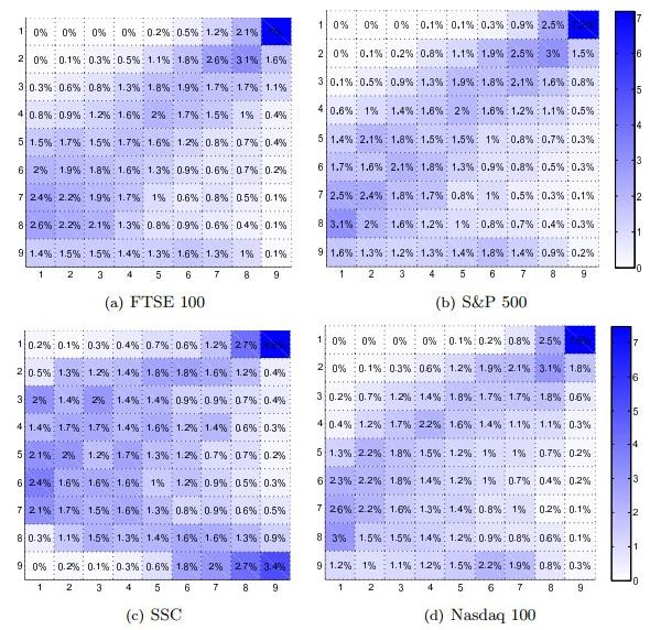
Figure 2 Joint frequency tables of the 90 days PDMA, , and realized volatility in the nest period. Panels report the percentage of each cell in the total number of observations |
Full size|PPT slide
The copula couples the marginal distributions together in order to constitute a joint distribution. The dependence relationship is well described by the copula, while scaling and shape are determined by the marginals (see [
19]).
An important measure of the dependence of the variables at the extremes is called as tail dependence. The upper tail dependence parameter is the limit (if it exists) of the conditional probability that is greater than the -th percentile of given that is greater than the -th percentile of as approaches 1, i.e.,
where and are continuous random variables with distribution functions and , respectively.
Similarly, the lower-upper tail dependence parameter , which measure the probability that one variable is extremely larger given that another variable is extremely smaller, is defined as,
If
or
are positive, X and Y are said to be upper or lower-upper tail dependence. These parameters depend only on the copula of
and
, as the following equation demonstrates, see [
19,
20].
Since the of and are equal to the of and , we have the following similar conclusion:
Different copulas usually delineate different dependence structure with a so-called association parameter, , which indicates the degree of the dependence. To investigate the dependence structure of the PDMA on the future volatility of stock indexes, we employ a linear combination of the Gumbel copula and its semi-rotated version (semi-survival Gumbel), since the copula tables show some evidences of upper and lower-upper tail dependence in the PDMA and volatility. We use the Gumbel copula for the upper tail dependence in order to assess whether a large positive PDMA is followed by high volatility2 The Gumbel copula is
2We adopt Gumbel type copula referring to the existing literature [
21]. In their studies, they use Gumbel type copula to investigate the tail dependent between realized volatilities and return.
The upper tail dependence parameter of Gumbel copula is . We apply the semi-survival Gumbel copula for the low-upper tail dependence in order to assess whether a large negative PDMA is followed by high volatility. The semi-survival Gumbel is given by
The lower-upper tail dependence parameter of semi-survival Gumbel copula is . The mixture of Gumbel and semi-survival copula, CMG, has equal to
This specification allows asymmetries between upper and lower-upper tail dependence. The parameter is the mixing parameter, while the upper and lower-upper tail dependence of CMG are and .
Similar to Patton
[22] and Hafner and Manner
[23], among others, we extend the CMG (Equation (9)) to that allows the tail dependence to vary with the time. We assume that the mixing parameter remains fixed over the sample period whereas the dependence parameters of the copula varies according to some evolution equations. We propose the following ARMA type process for the innovation of tail dependence parameters.
where, and are the logistic transformation of the tail dependence parameters. And
The right-hand side of the model contains an autoregressive term designed to capture the persistence in the dependence, and a forcing variable. As Patton
[22] pointed out, identifying a forcing variable for a time-varying limit probability is somewhat difficult. We propose to define new variables,
and
, to measure distances of
and
from extreme value 1, and using their mean over the previous
observations as a forcing variable. The expectation of this distance measure is inversely related to the concordance ordering of copulas at the extreme; when
approach to 1 simultaneously, the value of
is close to zero.
To avoid any distortion from the parametric assumption of marginal distributions, we employ a nonparametric method for the marginal distributions of the PDMA and the realized volatility. In this study, we use the empirical cumulative function (ECDF) for the margins. The ECDF of the PDMA and the realized volatility are calculated by kernel way. Finally, a maximum likelihood approach is employed to estimate the joint copula models.
3 The Data and Empirical Analysis
3.1 The Data
Our data set consists of close price, returns and realized measures for eight main stock market indexes including the S & P 500 index et al (listed in
Table 1). The data are provided by the database 'Oxford-Man Institute's realized library' version 0.2, which has been produced by Heber, et al.
[24]3. For each asset the library records daily returns, close price, daily subsampled realized variances, daily realized kernels, etc. We adopt the realized kernel, introduced by Barndorff-Nielsen, et al.
[16], as the realized measure,
, and define
as realized volatility,
. The close price
4 of each asset are used to compute the PDMAs by Equation (1) with the given periods of 10, 20 and 90 trading days that can be viewed as short-term, medium-term and long-term PDMAs respectively.
Table 1 Summary Statistics for the variables |
| asseta | D10, t | | D20, t |
| | mean | std. | skewb | kurt | mean | std. | skew | kurt |
| S&P | 2.20/104 | 0.020 | -1.184 | 9.647 | | 4.92/104 | 0.028 | -1.487 | 9.416 |
| DJIA | 3.62 /104 | 0.019 | -1.092 | 9.376 | | 7.77 /104 | 0.027 | -1.333 | 8.553 |
| Nasd | - 1.25/104 | 0.027 | -0.895 | 7.173 | | - 2.08 /104 | 0.040 | -1.178 | 6.587 |
| Nikkei | - 5.25 /104 | 0.025 | -0.918 | 8.307 | | - 1.04 /103 | 0.037 | -1.008 | 7.584 |
| FTSE | - 1.12 /104 | 0.019 | -1.042 | 8.062 | | - 1.81 /104 | 0.027 | -1.350 | 7.893 |
| DAX | 2.16 /104 | 0.026 | -1.088 | 7.534 | | 4.79/104 | 0.037 | -1.393 | 7.434 |
| H S | 1.34 /104 | 0.028 | -1.267 | 24.47 | | 4.24 /104 | 0.040 | -1.273 | 17.719 |
| SSC | - 1.87 /104 | 0.028 | -0.276 | 4.426 | | - 3.97/104 | 0.043 | -0.237 | 3.929 |
| asset | D90, t | | RVt |
| | mean | std. | skew | kurt | mean | std. | skew | kurt |
| S&P | 2.27/103 | 0.060 | -1.690 | 7.910 | | 9.38/103 | 6.16/103 | 3.315 | 24.487 |
| DJIA | 3.94/103 | 0.054 | -1.542 | 6.872 | | 9.15/103 | 5.96 /103 | 3.622 | 28.002 |
| Nasd | - 1.67/103 | 0.089 | -1.407 | 5.477 | | 1.04 /102 | 6.82 /103 | 2.469 | 13.845 |
| Nikkei | - 4.77/103 | 0.084 | -0.699 | 5.395 | | 9.79 /103 | 5.07 /103 | 3.071 | 20.680 |
| FTSE | - 3.20/104 | 0.053 | -1.436 | 6.700 | | 8.28 /103 | 5.14/103 | 2.473 | 13.667 |
| DAX | 1.97/103 | 0.082 | -1.448 | 5.753 | | 1.18/102 | 7.29 /103 | 2.577 | 14.809 |
| H S | 2.50 /103 | 0.089 | -1.199 | 8.578 | | 8.61/103 | 4.54 /103 | 3.673 | 31.250 |
| SSC | - 2.48/103 | 0.109 | 0.077 | 3.762 | | 1.08/102 | 6.13 /103 | 1.879 | 8.304 |
| a S&P, DJIA and Nasd are Standard & Poor's 500 index, Dow Jones industrial average index and Nasdaq 100 index respectively, Nikkei is Japan's Nikkei 225 index, FTSE is FTSE 100 index of London Stock Exchange, DAX is German's Deutscher Aktien index, H S is Hang Seng index of Hong Kong stock market and SSC is the Shanghai (Security) Composite index.
b skew and kurt are skewness and kurtosis respectively. is realized volatility. |
3The data are available at the web site:
WWW.oxford-man.ox.ac.uk.
4The data are available at Yahoo Finance and the web site:
https://finance.yahoo.com/quote.
Table 1 gives summary statistics for the realized volatility and the PDMAs for each asset. The serious left skewness of the distribution of PDMA was confirmed by the Table 1 for all indexes excepting the SSC. As reported in Table 1, with increase of the given period of the PDMA, its standard variance grows larger and its kurtosis decreases. This indicates that the size of PDMA grows when its given period increases.
3.2 Dependence Results and Information for Future Volatility
Following Knight, et al.
[10], we construct an empirical copula table in order to snoop into the dependence structure in the data. Firstly, we rank both the PDMA and the next period realized volatility series in ascending order and, then, we divide each series evenly into 9 bins. Bin 1 includes the observations with the lowest values and bin 9 includes the observations with the highest values. Thus, we obtain the cells,
, for pairs of the PDMA and the future period realized volatility (
). Cell,
, includes the observations of pairs
and
which belong to bin
and bin
respectively. Secondly, we count the numbers of observations that are in cell
and form an empirical copula table. The dependence information can be deduced from the frequency table as follows: If the two series are perfectly correlated, most observations should lie on the diagonals; if they are independent, then the numbers in each cell will be about the same; if there is a positive lower (or upper) tail dependence between the two series, we would expect more observations in
(or
). Similarly, if a lower-upper (or upper-lower) tail dependence exists, we would expect to see a large number in
(or
).
Figures 1 and 2 report the dependence structure for S & P 500, Nasdaq 100, FTSE 100 and the SSC index (the similar results for the rest of the stock indexes are not presented for brevity). The number in cell of first panel is . This means that out of 3567 observations, there are 4.3 percentage of occurrences when the short-term PDMA () of FTSE 100 index lie in its lowest 9th percentiles and its next period volatility lay in its highest 9th percentiles. This number is much larger than the numbers in all of the other cells of first panel. And similar results can be observed in rest panels. We take this as the evidence of the lower-upper tail dependence. Additionally, the volatility of the highest 9th percentiles mostly lie in cell except for for all stock indexes. This can be viewed as the evidence of the upper tail dependence. These suggest that a large PDMA, especially large negative PDMA, is likely to be followed by high volatility. Overall, joint frequency tables in Figures 1 and 2 show strong evidence of the dependence between technical indicator and future volatility at extremes for these stock indexes.
A second evidence from Figures 1 and 2 is that the impacts of the moderate PDMA on volatility is not significant. As shown from each panal of figures, the volatility of lower percentiles tend to lie in cell that include moderate PDMA. This implies that the relationship between the PDMA and future volatility are very weak at normal markets.
In Table 2, we report the estimates of the mixture copula CMG (Equation (9)) for 3 given horizons of PDMA and 8 stocks indexes. As shown from the table, there exists both significant and positive lower-upper and upper tail dependence between the PDMA and the next period volatility in most of the cases. In short-term PDMA () cases, the estimates of the lower-upper tail dependence parameters is 0.3279 for S & P 500 index, while their upper dependence parameters is 0.0408. This means that when the technical indictors, PDMA (), is extremely small, that is, a large negative price deviation from MA, the probability that the volatility will be extremely high in the next day is about 33%, and when is extremely large, the probability is about 4%. This is consistent with the results of copula table in Figure 1b. Although there is some distinction in the estimated results between each stock index, the tails dependence are significant for 8 indexes. This indicates that the PDMAs are highly informative on the next day volatility at extremes.
Table 2 Static tail dependence |
| assets | | | | | |
| | | | | | | | |
| S&P | | | | | | | | | | | |
| DJIA | | | | | | | | | | | |
| Nasd | | | | | | | | | | | |
| Nikkei | | | | | | | | | | | |
| FTSE | | | | | | | | | | | |
| DAX | | | | | | | | | | | |
| H S | | | | | | | | | | | |
| SSC | | | | | | | | | | | |
| Note. and are the upper tail dependence parameter and the low-upper tail dependence parameter respectively, and mixing parameter. Reported in parentheses are the -statistics based on Newey-West standard errors. and indicate significance at 1% and 5% level respectively. |
From the estimates of the tail dependence parameters and and mixing parameter , there are interesting new empirical findings: Firstly, the lower-upper tail dependence parameter is larger than upper tail dependence parameter significantly and the mixing parameter is lower then 0.5 in most cases considered, confirming a strong asymmetric tail dependence. This suggests that the information contents of PDMA appears to be significantly asymmetric for all stock indexes excluding SSC. In other words, the volatility is more prone to be boosted up when the current prices go extremely far below the MA than when they go above MA. This can be explained by the fact that the large negative PDMA are observed more frequently on bear markets and the positive one are observed more frequently on bull markets. Generally, the volatility on bull markets are far lower than it on bear one. Secondly, the upper tail dependence will fade away, and the lower-upper tail dependence will enhance, as given horizons of PDMA increase in Europe and America cases. Finally, there are some distinct differences between emerging market indexes and developed market indexes in the dependence structure. As above mentioned, there is an asymmetry in developed market cases, while it is not detected significantly in SSC cases. Additionally, evanescence of the upper tail dependence do not appear as given horizons of PDMA increase in SSC cases. This may be due to its feature that investment from individual investors account for a large fraction of market capitalization and individual investors apt to behave irrationally at Shanghai market; meanwhile it lacks facilities for making shorts. Obviously, these new empirical finding will make sense for related fields.
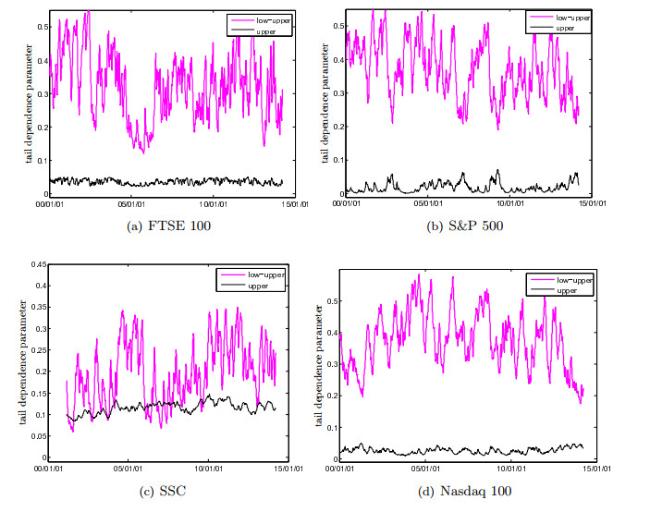
Next, we report the results of the time-varying tail dependence between future volatilities and the technical indictors (PDMA), in Table 35. The autoregressive coefficients are close to 1 and statistically significant, meaning strong persistence of both lower-upper and upper tail dependence. The estimated coefficient of forcing variable is significant and positive in lower-upper tail dependence, while the results are mixed in upper tail dependence. This result points on a type of mean-reverting behavior in lower-upper tail dependence, since the forcing variable is inversely related to the concordance ordering of copulas at extreme. This behavior can be observed and confirmed in Figure 3 as well. The significance of the dynamic parameters implies that the information content of the PDMA about future volatility is changing over time in some mean-reverting manner.
Table 3 Dynamic tail dependence |
| assets | | | |
| | | | | | | |
| S&P | | | | | | | | | |
| DJIA | | | | | | | | | |
| Nasd | | | | | | | | | |
| Nikkei | | | | | | | | | |
| FTSE | | | | | | | | | |
| DAX | | | | | | | | | |
| H S | | | | | | | | | |
| SSC | | | | | | | | | |
| Note. and are the parameters governing the time variation of the tail dependence. Reported in parentheses are the -statistics based on Newey-West standard errors. and indicate significance at 1% and 5% level respectively. |
5As shown in Table 2, the upper tail dependence is insignificant in 90-day given horizon cases (), so we only report results of and .
Figure 3 Dynamic impact on volatility from the first-order lag 20-days PDMA, . The figures plot the variation of the upper tail and lower-upper tail dependence coefficient against 09:50:57 |
Full size|PPT slide
To visually evaluate how degree of the information contents is changing over time, we plotted its dynamic pattern (with ) in Figures 3 for 4 indexes and took them as representative. As shown in the graphs, the tail dependence parameters fluctuate around their means, showing a volatile as well as persistent pattern over time. And their mean, by a rough estimate, is close to their estimated value in the static models.
4 Conclusion
In this paper, we investigate the information of the technical indicator (PDMA) on volatility in the next trading day for 8 stock indexes, where the volatility is measured by daily realized volatility. We first propose the static and dynamic copulas to model the impact by using tail dependence parameters to measure the amount of the information. The advantage of employing the copula approach for the evaluation of the dependence is that that it can conveniently separate the impact from their marginal distributions. The empirical analysis results imply that although there is some distinction in the estimated results between each stock index, the PDMAs are significantly informative on the next day volatility at extreme markets, while are less informative at normal markets for 8 indexes considered. We also find that: 1) The amount of information is asymmetric significantly in most case; 2) The information from positive PDMA will fade away, and that from negative one will enhance, as given horizons of PDMA increase in Europe and America cases; 3) There are some distinct differences between emerging market indexes and developed market indexes in the information contents. Moreover the information contents are found to be changing over time in a highly persistent manner. Although both the static and dynamic models can describe the leverage effect in the stock indexes, we find that the latter performs better than the former.
It is shown that the information varies with the given period of the PDMA. Thus, understanding given periods and the kind of moving averages that capture the information as best as possible is another interesting problem. This is left for future research.
{{custom_sec.title}}
{{custom_sec.title}}
{{custom_sec.content}}
 PDF(283 KB)

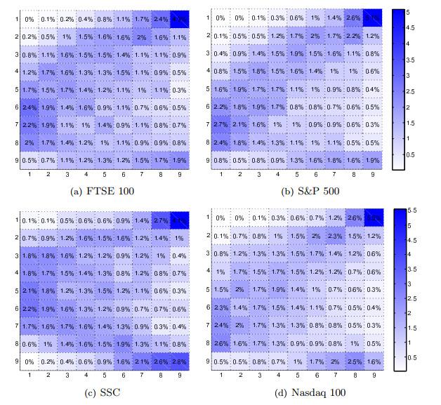
 Figure 1 Joint frequency tables of the 10 days PDMA,
  Table 1 Summary Statistics for the variables


