1 Introduction
The issue of stock market fluctuation has been a problematic problem in the field of financial economics studies. Traditional financial economic pricing models such as CAPM and APT models do not perform satisfactorily in empirical tests because such models are usually based on certain basic assumptions (e.g., investors are completely rational, maximizing utility; investors have homogeneity and the same expectation for the future earnings of the same securities; and there is no arbitrage limitation in the market). However, some studies suggest that investors' decision-making processes are not based entirely on achieving maximum utility; even if they are, sufficient rationality and ability to achieve this goal is hard to meet. Camerer and Fehr
[1] argued that investors have incomplete rationality or self-interest. Benartzi and Thaler
[2] noted that investors mechanically averaged and diversified investments within a selective range. Hu
[3] postulated that compared with individual company reports, financial reports on groups of companies are more difficult to understand, and therefore stock prices react more slowly to earnings information regarding the latter. Moreover, the assumption of investor homogeneity is difficult to satisfy. Kumar, et al.
[4] refered to the influence of religious culture on investment decisions. Grinblatt, et al.
[5] indicated that high IQ investors exhibit more accurate investment judgment. Cronqvist, et al.
[6] highlighted the influence of the living environment on investment style. In addition, some studies show that arbitrage restrictions exist, for example, Lamont and Thaler
[7] argued that short selling restrictions are one of the main causes of mispricing, while Gabaix, et al.
[8] noted that arbitrage restrictions are particularly evident in markets with high demand for expertise. For these reasons, stock price fluctuations in the short run are difficult to predict effectively. In the long run valuable information will gradually circulate in the market and be effectively absorbed. When the market realizes that a stock price deviates from its intrinsic value, it will act to correct the price, and this is reflected in the long-term mean reversion phenomenon. There are two research approaches for examining mean reversion. One holds that there is a negative autocorrelation in time series data for stock returns, and a negative autocorrelation indicates that there is a mean reversion for returns. Fama, et al.
[9] in their test of stock data on the New York Stock Exchange from 1926 to 1985 found a significant negative autocorrelation of stock returns over a period of more than one year. Jegadeesh
[10] stated that both the US and UK stock market index returns had a significant seasonal mean reversion effect in January. Lakonishok, et al.
[11] found that the future returns from holding high-growth stocks tend to be lower than the returns from holding low-valuation stocks. This phenomenon indicates that there is a mean reversion of stock returns. Daniel, et al.
[12] noted that the stock's positive return will be accompanied by a long-term correction process (reversal); that is to say, there is mean reversion in stock returns. Balvers, et al.
[13] uncovered that there is a mean reversion in stock market index returns, with an average return cycle of 3 to 3.5 years. Song
[14] observed that the monthly income of the Shanghai Composite Index exhibits a significant mean reversion feature. Zhao
[15] in tests on the daily return rate of stocks in Shanghai and Shenzhen stock markets from 1996 to 2003 indicates that the market return time series still exhibits mean reversion even after risk adjustment. He
[16] argued that the Shanghai stock market, whether in a bull or bear market, showed mean reversion in the time series of stock returns. Dai
[17] noted from a regression analysis of the daily trading data of index and individual stocks in Chinese and US stock markets from 1990 to 2014 that the mean reversion cycle of China's stock market returns is less than one year, while in the US stock market it is 1
2 years. The alternative view, articulated by Campbell, et al.
[18], is that the relative value of the stock market cannot be accurately measured, but it can be represented to some extent by the index valuation ratio. They found that between 1871 and 2000, the price/earnings ratio of the S & P 500 crosses, on average, the mean value once every 4.78 years, and the dividend/price ratio on average once over 4.45 years. Hirshleifer
[19] indicated that stock pricing is related to risk and also affected by market valuation level, which is associated with individual investor's psychological attitude, and valuation level approach the mean over the long term. Huang, et al.
[20] found that in any stock market, the price-earnings ratio experiences a gravitational pull toward the mean. Ma
[21] noted that a time series of the index price-earnings ratio in the Shenzhen Composite B-share Index exhibits mean reversion. Wang
[22] stated that stock prices that deviate from their intrinsic value eventually converge toward their intrinsic value in their study of stock market trends following eight financial crises. Chang, et al.
[23] documented a strong negative correlation between historical high valuation positions and trends for subsequent stock indexes through their empirical research on G7 national stock markets. Those results present evidence that there is mean reversion in stock markets. Mean reversion theory provides an effective perspective from which to learn about stock market fluctuation in the long term. In this paper, the method based on Campbell, et al. will be used to study a larger sample, including different markets, to examine if there is a general law in stock markets. Our study is based on data of 10 stock markets indexes during 2000 to 2018. Following Campbell, et al., we select variables of relative price of the stock market such as price/earnings ratio and dividend ratio, then define the mean value of them as the intrinsic value. We empirically examine whether mean reversion law is universe in most stock markets. The empirical analysis documents that the relative price fluctuates around the intrinsic value in the long term, and the relative price approximately approaches the intrinsic value once in 3 to 4 years. Prior studies note that valuations of the stock market can be used to predict price fluctuation in the subsequent years in some extent (Campbell, et al.
[33]). And Mulligan and Lombardo
[24] demonstrated that most investors ignore the vast majorities of relevant information, until it accumulates a critical mass they must finally recognize, and they attempt to compensate for their history of informational sloth. Adra, et al.
[25] showed evidence that although overvaluation stock investors don't experience significant announcement period price falling, they receive negative returns in the post-announcements period. Itemgenova and Sikveland
[26] showed that stock return on stock market is negatively associated with the price-earnings ratio. Dergiades, et al.
[27] postulated that both price-earnings ratio and dividend ratio can affect stock market returns at long and short horizons. Besides, dividend-price ratio can represent the relative valuation of stock price at some extent. As Khanal and Mishra
[28]; Esteve, et al.
[29]; Bask
[30] argued that stock price responds positively to the announcements of change in dividend ratio, and the pure dividend announcement effect is the immediate change in the stock price and the time effect is the cumulative change in the stock price. Those literatures document that stock market respond to the change of valuations by adjusting the price in the subsequent period. Furthermore, by merging the data of individual market into a pool sample, we test the relationship between current relative price of the stock market and the price growth rate in the subsequent 1 to 3 years. We find that the current Price/Earnings ratio of the index has a negative coefficient to the price growth in the subsequent 1 to 3 years. This result indicates that the growth of stock price tends to be inhibited by the current high Price/Earnings ratio. Dividend ratio of the index, which is negatively associated with the Price/Earnings ratio, has a positive regression coefficient to growth rate of the price in the subsequent 1 to 3 years. This result indicates that the price growth in the future 3 years is stimulated by the high dividend ratio. Our analysis uncovers a mechanism that the stock market can adjust the price fluctuation by the level of valuation. When the current market has run to a high level which is measure by the valuation ratio, price growth rate in the subsequent years is tend to be inhibited, in contrast, when the market drop in a low level which is measured by the valuation of the market, stock price growth in the subsequent years is tend to be stimulated. And thus, the relative value of stock market fluctuates in a proper range and it will not deviate too far from the fundamental value in the long term.
The rest of the paper is structured as follows. In Section 2 we show the research design and data. In Section 3 we examine whether mean reversion is a universe law in most stock markets. In Section 4, we test the relationship between current valuation ratio and the growth rate of price in the subsequent years. Section 5 is the robustness check. And in Section 6 we conclude the paper.
2 Research Design and data
2.1 The Research Route
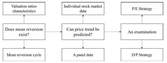
As shown above, the study's main contents are divided into three parts. The first mainly verifies whether there is a "mean reversion law" in the stock market and covers two tasks: (ⅰ) To verify that valuation ratios fluctuate around the mean value and (ⅱ) estimate the mean reversion cycle. The second examines whether valuation ratios can predict price fluctuation in the future. Finally, according to the mean reversion law and the relationship between valuation ratios and stock price trends, two quantitative investment strategies are constructed to test whether mean reversion theory is effective.
Figure 1 The research route |
Full size|PPT slide
2.2 The Data
It should be noted that emerging markets now represent a large share of the global stock market, and their importance cannot be ignored. In addition, only studying developed markets or emerging markets cannot effectively demonstrate the universality of any law on stock market volatility. Therefore, in this paper, 10 stock markets, including 6 developed markets and 4 emerging markets, are selected as research objects. We select 10 stock market indexes from the Americas, Asia, Australia, and Europe. The nature of the market is based on the MSCI Emerging and Developed Market Index. The data period extends from 2000 to 2018, and while there are missing individual years due to invalid data processing, this should not affect the overall estimation results. Our data resources are from Bloomberg and wind.
Table 1 Information on the index |
| Country | Index | Market Nature |
| United States | SP500 Index | Developed |
| Canada | SPTSX Index | Developed |
| Mexico | MEXBO Index | Emerging |
| The UK | FTSE Index | Developed |
| Germany | DAX30 Index | Developed |
| Australia | AS51 Index | Developed |
| Japan | N225 Index | Developed |
| Thailand | SET Index | Emerging |
| China | Shanghai Composite Index | Emerging |
| China | TWSE Index | Emerging |
3 Does Mean Reversion Exist?
3.1 Research Design
3.1.1 Period Covered by the Ratio
Benartzi, et al.
[31] contend that it is difficult to have an investment evaluation period that is suitable for every investor. However, if one must choose a reasonable period, one year is appropriate. For individual investors, tax returns are required each year, comprehensive reports from their brokerage firms, mutual funds and pension accounts are received once a year, and institutional investors take annual reports very seriously. Therefore, the basic period for the variables is set at 1 year.
3.1.2 Relative Price of the Stock Market
In the stock market, the price/earnings ratio is used to measure the relative price level of stocks. It is one of the most frequently used indicators by investors and in analyst research reports. The price-earnings ratio indicator in this paper is defined as the year-end market value relative to the profit value of the year: , referred to as P/E. The relative price indicator could be formulated as: .
The dividend/price ratio is an important indicator to evaluate whether a stock has investment potential. Becker
[32] argued that dividend yield is an important factor for investors to consider when making investment decisions. The dividend/price indicator in this paper is defined as the dividend to market value:
, referred to as D/P. Another relative price indicator is:
.
3.1.3 Intrinsic Value
It is hard to evaluate the intrinsic value of stock market precisely, but as Campbell, et al.
[18] reviewed that the intrinsic value could be represented by the mean value of valuations ratios in some extent, let
and
denote the intrinsic value:
,
.
3.1.4 The Cycle of Mean Reversion
The method to detect the mean reversion is calculating the difference between the adjacent year that the relative price crossing the intrinsic value: . And the average cycle in market is .
3.1.5 Fluctuation Range of Stock Market
The relative deviation of the valuation ratio is defined as following, denotes the mean value of P/E in market , with periods, the P/E in period market is defined as , and the average deviation of P/E in market over periods is denoted as: ; The mean value of D/P in market is , with periods, and the D/P in period market is defined as , with the average deviation of P/E for market over periods: . indicates the distance of P/E and D/P from the mean value.
3.2 Empirical Research
3.2.1 Mean Reversion
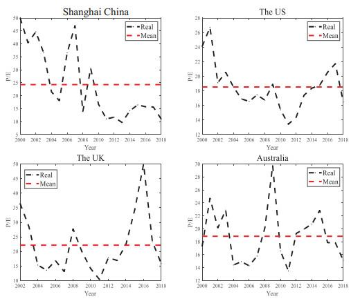
In the P/E ratio data, some values are too large in individual years, and the first 5 quantile (50) is used as an upper limit of the P/E ratio to eliminate the influence of extreme values. The data in four markets is plotted in Figures 2 and 3, with more details in Tables 2 and 3.
Figure 2 The volatility of P/E |
Full size|PPT slide
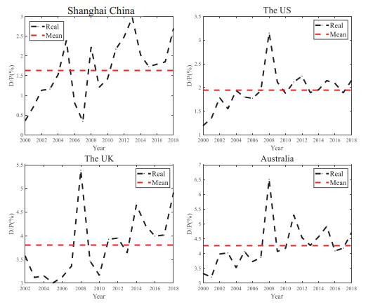
Figure 3 The volatility of D/P |
Full size|PPT slide
Table 2 Descriptive statistics of P/E |
| Index | MEAN | Std dev | Average cycle(year) | Std dev(year) |
| SHCI | 25.07 | 15.63 | 3.60 | 4.72 |
| TWSE | 13.18 | 2.78 | 3.00 | 2.00 |
| SP500 | 18.53 | 3.22 | 3.60 | 1.67 |
| SPTSX | 19.55 | 3.87 | 3.60 | 1.52 |
| MEXBO | 18.5 | 5.40 | 9.00 | 2.83 |
| FTSE100 | 22.31 | 10.80 | 3.40 | 1.95 |
| DAX30 | 32.56 | 52.05 | 3.20 | 1.48 |
| N225 | 28.90 | 18.28 | 3.60 | 4.72 |
| AS51 | 18.85 | 4.16 | 3.00 | 0.89 |
| SET | 14.80 | 3.10 | 2.29 | 1.70 |
| MEAN | 21.23 | 11.93 | 3.83 | 2.34 |
Table 3 Descriptive statistics of D/P |
| Index | MEAN | Std dev | Average cycle(year) | Std dev(year) |
| SHCI | 1.63 | 0.77 | 3.60 | 4.72 |
| TWSE | 3.44 | 1.55 | 2.57 | 2.44 |
| SP500 | 1.94 | 0.40 | 2.57 | 2.51 |
| SPTSX | 2.52 | 0.75 | 6.00 | 7.81 |
| MEXBO | 1.71 | 0.49 | 2.57 | 1.51 |
| FTSE100 | 3.80 | 0.68 | 3.20 | 3.83 |
| DAX30 | 2.85 | 0.81 | 2.43 | 1.81 |
| N225 | 1.44 | 0.55 | 6.00 | 5.57 |
| AS51 | 4.27 | 0.75 | 3.60 | 2.88 |
| SET | 3.52 | 1.13 | 2.00 | 1.41 |
| MEAN | 2.77 | 0.80 | 3.36 | 3.36 |
3.2.2 Results Analysis
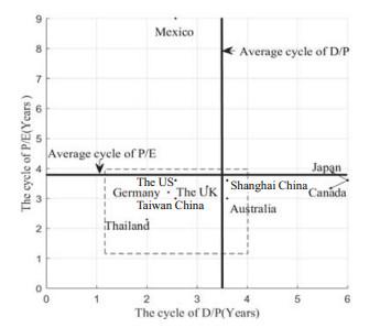
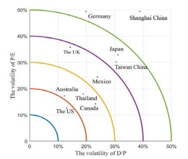
Figure 4 shows the mean reversion periods for P/E and D/P in different stock markets. On average, the P/E cycle in our 10 markets is 3.83 years, and the D/P cycle is 3.36 years. In most markets, the average time required for the valuation ratios to cross their own mean values once is less than 4 years. However, the P/E cycle of the Mexican market is 9 years, far above the international average, and the D/P ratio in the Japanese and Canadian markets is between 5 and 6 years, which substantially exceeds the international average. If the mean reversion cycle is long, this indicates that the market needs a longer period to adjust the relative value to a reasonable level, and reflects a limited ability to adjust itself; If the mean reversion period is short, this indicates that once the relative value deviates from the reasonable level, the adjustment mechanism will act faster to push the price back to a reasonable level. We also exhibit the level of relative price deviation from the intrinsic value in different stock markets in Figure 5. The US stock market's average deviation is less than 20, Australia, Thailand and Canada are less than 30, the UK and Mexico are less than 40, France, Taiwan China, Japan and Spain are less than 50, and Germany, Brazil and Shanghai China are more than 50. Those results indicate that although stock price deviate from the intrinsic value in different degrees in individual market, the relative price fluctuates around the intrinsic value and approaches it on average once in 34 years.
Figure 4 Mean reversion cycle |
Full size|PPT slide
Figure 5 The Fluctuation range |
Full size|PPT slide
4 Could Valuation Ratios Forecast the Growth of Index Price?
4.1 Theoretical Analysis and Model Design
4.1.1 Theoretical Analysis
According to the analysis above, we demonstrate that the P/E and the D/P are subject to the mean reversion law. As Campbell and Shiller
[18] argued that in the long run, valuations that are high will inevitably decline, and those that are low will eventually rise. Campbell, et al.
[33] showed that the volatility of the index price over the next 1
5 years can be predicted by stock market valuations to a certain degree. Mulligan and Lombardo
[24] demonstrated that most investors ignore the vast majorities of relevant information, until it accumulates a critical mass they must finally recognize, and they attempt to compensate for their history of informational sloth by overreacting. Itemgenova and Sikveland
[26] showed that return on stock market is negatively related to the price-earnings ratio. Dergiades, et al.
[27] postulate that price-earnings ratio and dividend affect stock market returns at long and short horizons. Combining those literatures with mean reversion law, it is reasonable to hypothesize that when price-earnings ratio climb to a high level, stock price tends to decline or grow more slowly to push the price-earnings ratio down. According to this, we propose hypothesis H1.
Hypothesis H1 A high current P/E ratio will inhibit index price growth in the next mean reversion cycle. On the other hand, dividend-price ratio can represent the relative valuation of stock price at some extent.
As Ross
[34] contended that investors regard a company's dividend policy changes as expected changes in future earnings prospects. If investors incorporate this policy change into their investment decisions, then the dividend/price rate should be related to future market changes. Khanal and Mishra
[28] argued that stock price responds positively to the increase of dividend. Esteve, et al.
[29] postulate that since the announcements of increase in dividend, the stock price reacts to changes in dividends over a long time. Bask
[30] contends that the pure dividend announcement effect is the immediate change in the stock price and the time effect is the cumulative change in the stock price. Those works contribute the conclusion that stock price shall adjust to the change in dividend in the subsequent period. As dividend fluctuate around the mean value in the long run, it is reasonably to assume that when dividend ratio is high, price growth shall be high to balance the ratio. According to this, there we have hypothesis H2.
Hypothesis H2 A high current D/P ratio will stimulate price to increase in the next mean reversion cycle.
4.1.2 Econometric Model Design
Based on panel data composed of 10 markets between 2000 and 2018, we build the econometric models to estimate the influence of earnings/price or dividend/price to market price growth in subsequent years. To be specific, as Conrad
[35] contend that stock prices have different responses to favorable information under different relative valuation levels.
and
are defined as the relative ratio of P/E and D/P:
,
; let
denotes the profit growth rate from year
to year
. Besides, sentiment influences the return of stock prices Baker
[36]. Controlling variables such as growth rate of earnings, value of the stock market, nature, and size are also taken into consideration in the econometric model.
represents the trading sentiment of year
, defined as the logarithm of the turnover rate.
is the overall market index value in year
,
is the market size, divided into three categories, where the smaller the number is, the larger the size.
is a dummy variable indicating the nature of the market, where 0 is a developed market, and 1 represents emerging market. Let
denote a random disturbance term. The explained variable
is defined as the growth rate from year
to year
in market
:
, where
is the value in period
of market
,
is dividend in year
of market
.
In practice, a high price growth rate may also be an influence of the P/E and D/P, and there may be mutual influences between explanatory variables. In order to eliminate the endogenous problem, Ⅳ (instrument variable method) is chosen, and different estimation methods are also used to compare results. The statistics of main variables are shown below. As we can see, the mean of explanatory variable is 0.97, and it ranges from 0.34 to 7.32, the mean of the variable is 1.02, and it ranges from 0.28 to 2.42. The mean of the explained variable is 0.11, and it ranges from 0.52 to 1.57. And for another explained variable , the mean is 0.41, it ranges from 0.51 to 1.88. Besides, the mean of is 0.25, the variable ranges from 0.67 to 6.60. The mean of is 0.67, it ranges from 0.66 to 29.53.
Table 4 The statistics of main variables |
| Variable | Mean | Std.Dev. | Min | Max | Total |
| 0.11 | 0.27 | 0.52 | 1.57 | 158 |
| 0.25 | 0.71 | 0.67 | 6.60 | 158 |
| 0.97 | 0.61 | 0.34 | 7.32 | 158 |
| 1.02 | 0.29 | 0.28 | 2.42 | 158 |
| 0.41 | 0.45 | 0.51 | 1.88 | 140 |
| 0.67 | 2.61 | 0.66 | 29.53 | 140 |
4.2 The Results
4.2.1 The Impact of Valuation Ratios to the Price Growth in the Next Year
The impact of standard D/P. In
Table 5, we can see that after the
is added as an explanatory variable in the OLS regression equation, the
statistic rises from 6.81 to 10.08, and the
is 10.3
, indicating that
has an effect on price growth. However,
and price growth may influence one another, so that there may be endogeneity problems. The Hausman test results support the rejection of all hypotheses at the 1
significance level for the exogenous variables. Ⅳ method is used to eliminate endogeneity problems, and lagged variables of
and
were chosen as the instrumental variables of the core explanatory variable. The
value of the exogeneity test is 0.62, indicating that the instrumental variable is exogenous and has no relationship with the random disturbance term. Estimations using different methods are shown in
Table 5. After the use of the instrumental variables, the coefficient of
is slightly improved. The
regression coefficients calculated by the five estimation methods of OLS, TSLS, LIML, GMM, and IGMM have no substantial differences, and its coefficients are significant at the 1
level. The coefficient of
is approximately 0.28, consistent with prior theories such as
[28–30], which postulate that an increase in dividend will increase the return in the subsequent period. Our estimation indicates that for every 1
increase in the
, the price growth rate tends to rise by approximately 0.3
in the subsequent year. The coefficient of
is positive, consistent to findings such as Berggrun, et al.
[37], indicates that effect of profitability on stock price is positive. The coefficients of
is significant negative, which shows that the regulatory effect on valuations is less obvious in emerging markets. This result is consistent to prior works which argue that there is great difference between emerging markets and developed markets as Jin, et al.
[38] postulate. And coefficients of
and
are both negative, the coefficients indicate that that regulatory effect is different as size and capital value changes as Conard, et al.
[35] proposed.
Table 5 The impact of the standard D/P ratio on price growth |
| OLS no | OLS with | | | | |
| 0.108 | 0.110 | 0.114 | 0.114 | 0.127 | 0.134 |
| | (0.012) | (0.016) | (0.016) | (0.016) | (0.010) | (0.010) |
| 0.017 | 0.010 | 0.007 | 0.007 | 0.003 | 0.003 |
| | (0.261) | (0.481) | (0.630) | (0.620) | (0.820) | (0.830) |
| 0.076 | 0.078 | 0.058 | 0.058 | 0.054 | 0.054 |
| | (0.018) | (0.012) | (0.010) | (0.010) | (0.012) | (0.012) |
| 0.201 | 0.209 | 0.162 | 0.162 | 0.154 | 0.154 |
| | (0.025) | (0.013) | (0.011) | (0.011) | (0.013) | (0.013) |
| 0.441 | 0.0459 | 0.339 | 0.339 | 0.323 | 0.323 |
| | (0.010) | (0.005) | (0.002) | (0.002) | (0.002) | (0.002) |
| | 0.273 | 0.279 | 0.277 | 0.283 | 0.293 |
| | | (0.000) | (0.019) | (0.032) | (0.023) | (0.020) |
| 1.483 | 1.437 | 1.032 | 1.034 | 1.048 | 1.038 |
| | (0.049) | (0.042) | (0.055) | (0.056) | (0.048) | (0.049) |
| 158 | 158 | 149 | 149 | 149 | 149 |
| 18.3 | 28.6 | 33.5 | 33.5 | 33.3 | 33.2 |
| Notes: The first column is the OLS estimation result with no , the second column is the OLS estimation result when is added, the third column is the Ⅳ estimation result, the fourth column is the LIML estimation result, the fifth column is the GMM estimation result, and the sixth column contains estimation results using IGMM. And *** denotes 0.01, ** denotes 0.05, and * denotes 0.1. |
From
Table 6, we can see when adding
to the regression Equation (1), the
is 14
, the
statistic rises from 6.81 to 12, and the regression coefficient of
is significant at the 1
level. First, the Hausman test results show that not all variables are strictly exogenous at the 1
level. The robust endogeneity test indicates that the endogeneity of
could not be rejected at the 10
significance level. To eliminate endogeneity concerns, lag one period variables of
, and
was chosen as the Instrumental variable, 2SLS, LIML, GMM, and IGMM estimation was employed. The estimates are reported in
Table 5. It can be seen from the table that after adding the
indicator, the regression coefficient of e1 is significantly increased from 0.11 to above 0.21, while the regression coefficient of
is approximately
0.20, the negative coefficient is consistent with prior literatures such as Itemgenova and Sikveland
[26]; Rahman and Shamsuddin, 2019
[39]; Dergiades, et al.
[27] argue. Our estimations indicate that the current
increases by 1
, and the price growth rate tends to decline by approximately 0.2
.
Table 6 The impact of the standard P/E ratio on price growth |
| OLS no | OLS with | | | | |
| 0.108 | 0.266 | 0.354 | 0.954 | 0.291 | 0.209 |
| | (0.012) | (0.000) | (0.000) | (0.035) | (0.000) | (0.000) |
| 0.017 | 0.013 | 0.010 | 0.0036 | 0.005 | 0.0008 |
| | (0.261) | (0.330) | (0.425) | (0.906) | (0.685) | (0.956) |
| 0.080 | 0.060 | 0.050 | 0.007 | 0.001 | 0.028 |
| | (0.020) | (0.030) | (0.045) | (0.930) | (0.760) | (0.260) |
| 0.201 | 0.194 | 0.190 | 0.163 | 0.060 | 0.040 |
| | (0.025) | (0.017) | (0.014) | (0.205) | (0.389) | (0.600) |
| 0.441 | 0.421 | 0.410 | 0.334 | 0.108 | 0.127 |
| | (0.010) | (0.007) | (0.006) | (0.162) | (0.413) | (0.362) |
| | 0.213 | 0.331 | 1.139 | 0.256 | 0.166 |
| | | (0.000) | (0.000) | (0.387) | (0.000) | (0.000) |
| 1.483 | 1.550 | 1.587 | 1.839 | 0.445 | 0.395 |
| | (0.049) | (0.024) | (0.016) | (0.090) | (0.473) | (0.575) |
| 158 | 158 | 158 | 158 | 158 | 158 |
| 18.3 | 32.3 | 28.0 | - | 26.3 | 14.2 |
| Notes: The first column is the OLS estimation result with no , the second column is the OLS estimation result when is added, the third column is the Ⅳ estimation result, the fourth column is the LIML estimation result, the fifth column is the GMM estimation result, and the sixth column contains estimation results using IGMM. And *** denotes 0.01, ** denotes 0.05, and * denotes 0.1. |
The impact of cross-terms: In addition, adding to the equation that already contains , there is little difference between the results of OLS and Ⅳ estimation. models in (3) (4) (5) columns that add cross terms such as , , and , the coefficient of the cross term in (4) is 0.16, but it is not statistically significant at the 10 level. The coefficient of in (5) is 0.18, but it is not statistically significant at the 10 level. The cross term of in (5) is 0.01, and the effect is almost non-existent.
4.2.2 The Impact of Valuation Ratios to the Price Growth in the Next 3 Years
In order to examine whether the valuations have a regulatory effect on stock price growth during a longer period, we estimate the coefficients between valuations and stock price growth in the subsequent 3 years. We can see from the table below, the coefficient of
in the OLS method is 0.20, but in the
,
,
,
method, the regression coefficient is approximately 0.67, those results are still consistent with findings of
[28–30]. This positive coefficient indicates that for every 1
increase in the
, the price growth rate 3 years into the future tends to rise by approximately 0.67
.
Table 7 The impact of all variables on price growth |
| (1) | (2)(OLS) | (2)TSLS | (3) | (4) | (5) |
| 0.110 | 0.249 | 0.329 | 0.289 | 0.09 | 0.281 |
| | (0.016) | (0.000) | (0.000) | (0.000) | (0.440) | (0.000) |
| Control | Yes | Yes | Yes | Yes | Yes | Yes |
| 0.273 | 0.226 | 0.199 | 0.236 | 0.175 | 0.238 |
| | (0.000) | (0.000) | (0.002) | (0.000) | (0.007) | (0.000) |
| | 0.188 | 0.295 | 1.154 | 0.197 | 0.160 |
| | | (0.000) | (0.000) | (0.000) | (0.000) | (0.000) |
| 1.437 | 1.504 | 1.542 | 1.490 | 1.490 | 1.490 |
| | (0.042) | (0.022) | (0.015) | (0.009) | (0.010) | (0.001) |
| | | | 0.155 | | |
| | | | | (0.157) | | |
| | | | | | |
| | | | | | (0.130) | |
| | | | | | 0.011 |
| | | | | | | (0.210) |
| 158 | 158 | 158 | 158 | 158 | 158 |
| 28.6 | 39.1 | 35.7 | 39.95 | 40.04 | 39.77 |
| Notes: The first column is the OLS estimation result with no , the second column is the OLS estimation result when is added, the third column is the Ⅳ estimation result, the fourth column is the estimation result with , and the fifth column contains the estimated results with . The sixth column contains the estimated result with . And *** denotes 0.01, ** denotes 0.05, and * denotes 0.1. |
The impact of P/E in the subsequent 3 years: We can see from the table below that the coefficient of
in all estimation methods are negative. The coefficient using the Ⅳ estimation is approximately
0.74, which indicates that for every 1
increase in the
, the price growth rate in the following 3 years tends to decline by approximately 0.74
. The results are consistent with prior theories such as Itemgenova and Sikveland
[26]; Rahman and Shamsuddin
[39]; Dergiades, et al.
[27] propose. Comparing the coefficients of valuation and stock price growth between 1 and 3 years, it is found that the coefficients of
and
are larger in the latter, indicates that stock price have a persistent adjusting process in the subsequent period.
Table 8 The impact of the standard D/P ratio on price growth over 3 years |
| OLS no | OLS with | | | | |
| 0.030 | 0.029 | 0.028 | 0.028 | 0.028 | 0.028 |
| | (0.013) | (0.016) | (0.016) | (0.020) | (0.015) | (0.015) |
| 0.013 | 0.006 | 0.010 | 0.021 | 0.019 | 0.020 |
| | (0.592) | (0.781) | (0.508) | (0.443) | (0.440) | (0.431) |
| 0.102 | 0.103 | 0.093 | 0.092 | 0.094 | 0.093 |
| | (0.009) | (0.006) | (0.019) | (0.036) | (0.020) | (0.020) |
| 1.270 | 1.275 | 1.257 | 1.253 | 1.263 | 1.263 |
| | (0.000) | (0.000) | (0.000) | (0.000) | (0.000) | (0.000) |
| 1.640 | 1.652 | 1.612 | 1.608 | 1.61 | 1.608 |
| | (0.000) | (0.000) | (0.000) | (0.000) | (0.000) | (0.000) |
| | 0.204 | 0.631 | 0.796 | 0.647 | 0.655 |
| | | (0.006) | (0.001) | (0.005) | (0.001) | (0.001) |
| 5.450 | 5.440 | 5.398 | 5.301 | 5.449 | 5.449 |
| | | (0.006) | (0.001) | (0.005) | (0.001) | (0.001) |
| 140 | 140 | 131 | 131 | 131 | 131 |
| 61.40 | 63.60 | 54.1 | 45.2 | 53.3 | 52.9 |
| Notes: The first column is the OLS estimation result with no , the second column is the IOLS estimation result when is added, the third column is the Ⅳ estimation result, the fourth column is the LIML estimation result, the fifth column is the GMM estimation result, and the sixth column contains estimation results using IGMM. And *** denotes 0.01, ** denotes 0.05, and * denotes 0.1. |
Our estimations show that high current price-earnings ratio inhibits price growth in the subsequent 1 to 3 years, and this effect supports Hypothesis H1 at the 1 significance level. A high current D/P stimulates price growth in the subsequent 1 to 3 years, and this result supports Hypothesis H2 at the 1 significance level. In this empirical analysis, it is found that the stock market has a self-regulating mechanism, i.e., under the condition where other variables are controlled, a high valuation level has an inhibitory effect on increases in stock prices, and a low valuation level has a stimulated effect.
4.3 Quantitative Strategies: An Application of Mean Reversion
According to the mean reversion law of the D/P and the P/E ratios, two investment strategies are constructed. Strategy One is to buy the index when P/E is lower than and hold for , where , , denotes the average period of P/E's mean reversion time in market . Strategy Two is to buy the index when D/P is higher than and hold for , where , , denotes the average period of D/P's mean reversion time in market . The control group denotes the annualized return on holding the index over the period 2000–2018. The results are estimated in Table 10. The average annualized return of Strategy One is 8.18, which is 1.27 higher than the control group, and the average annualized return of Strategy Two is 14.92, which is 8.01 higher than the control group. This method is based on the mean reversion rule; under certain criteria, when the relative price is low, buy and strictly hold for a P/E's mean reversion cycle; at a higher dividend rate, buy and strictly hold for a D/P's mean reversion cycle. It is clearly shown that the return under the two strategies substantially exceeds the annualized return of simply holding the market index, which objectively proves the existence of the mean reversion law.
Table 9 The impact of the standard P/E ratio on price growth over 3 years |
| OLS no | OLS with | | | | |
| 0.030 | 0.092 | 0.185 | 0.226 | 0.148 | 0.576 |
| | | (0.000) | (0.000) | (0.000) | (0.000) | (0.000) |
| 0.013 | 0.017 | 0.024 | 0.0273 | 0.03 | 0.002 |
| | | (0.430) | (0.288) | (0.269) | (0.167) | (0.928) |
| 0.102 | 0.084 | 0.055 | 0.042 | 0.078 | 0.088 |
| | | (0.022) | (0.170) | (0.378) | (0.036) | (0.231) |
| 1.270 | 1.244 | 1.203 | 1.186 | 1.225 | 0.933 |
| | | (0.000) | (0.000) | (0.000) | (0.000) | (0.000) |
| 1.640 | 1.587 | 1.508 | 1.473 | 1.537 | 0.963 |
| | | (0.000) | (0.000) | (0.000) | (0.000) | (0.001) |
| | 0.262 | 0.661 | 0.837 | 0.482 | 1.002 |
| | | | (0.000) | (0.001) | (0.000) | (0.000) |
| 5.450 | 5.187 | 4.787 | 4.611 | 4.904 | 2.462 |
| | | (0.000) | (0.000) | (0.000) | (0.000) | (0.067) |
| N | 140 | 140 | 140 | 140 | 140 | 140 |
| 61.40 | 65.40 | 56.20 | 46.3 | 62.1 | |
| Notes: The first column is the OLS estimation result with no , the second column is the OLS estimation result when is added, the third column is the Ⅳ estimation result, the fourth column is the LIML estimation result, the fifth column is the GMM estimation result, and the sixth column contains estimation results using IGMM. And *** denotes 0.01, ** denotes 0.05, and * denotes 0.1. |
Table 10 Investment returns |
| Index | The Control Group | Strategy One | Strategy Two |
| SHCI | 14.5 | 13.24 | 21.84 |
| TWSE | 7.03 | 14.11 | 14.90 |
| SP500 | 3.75 | 17.20 | 12.60 |
| SPTSX | 4.58 | 7.71 | 11.39 |
| MEXBO | 10.53 | 11.21 | 7.91 |
| FTSE100 | 4.06 | 2.37 | 8.77 |
| DAX30 | 0.92 | 5.19 | 18.41 |
| N225 | 3.51 | 0.49 | 16.00 |
| AS51 | 5.41 | 9.30 | 17.5 |
| SET | 14.79 | 1.91 | 19.83 |
| Mean | 6.91 | 8.18 | 14.92 |
4.4 Robustness Check
In order to examine whether our analysis is robust. We construct a new measurement of relative price of the market. Prior evidence documents that both Price/Earnings ratio and Dividend ratio can represent the relative level of the market in some extent. Here, we try to construct a new measurement by constructing an equation which is the linear combination of Price/Earnings ratio and Dividend ratio as shown as , where , . We adjust the form of as the reciprocal of Dividend ratio, to make sure that the Dividend ratio changes in the same direction as the Price/Earnings ratio changes. We set by experience after standardizing and , and show the results estimated by OLS in the table below. It is shown that the coefficients of are both negative and significant in the two equations, those coefficients indicate that the relative level of the market has a significant stimulated effect on the growth rate in the next 1 to 3 years.
| when | when |
| 0.16 | 0.033 |
| | | (0.018) |
| 0.003 | 0.059 |
| | | (0.017) |
| 2.612 | 6.145 |
| | | (0.000) |
| 0.000 | 0.538 |
| | | (0.000) |
| 0.101 | 0.608 |
| | | (0.000) |
| 0.128 | 0.104 |
| | | (0.029) |
| 2.778 | 7.414 |
| | | (0.000) |
| 158 | 140 |
| 34.03 | 49.84 |
| Notes: *** denotes 0.01, ** denotes 0.05, and * denotes 0.1. |
5 Conclusion
According to a statistical analysis of ten stock markets, we demonstrate that the relative price of the stock market fluctuates around the intrinsic value in the long run. The relative price on average crosses the intrinsic value once for 3.6 years. Specifically, the P/E ratio on average completes a mean reversion cycle after 3.83 years, and the corresponding figure is 3.34 years for the D/P ratio. In addition, from the estimation of the econometric model, stock market price fluctuations in the next 13 years could be effectively predicted through current valuation ratios in some extent. A high current P/E ratio has a significant inhibitory effect on index price growth over the subsequent 1 to 3 years: For every 1 increase in standard P/E, the price tends to decline by 0.24%0.74% in next 13 years; a high current dividend yield has a significant stimulated effect on price index growth over the next three years: for every 1 increase in standard D/P, the price tends to rise by 0.280.67 in the next 13 years. By adjusting the nominal index price, the market can complete its adjustment of the relative price to within a reasonable range: When the valuation ratio substantially deviates from the intrinsic value, the price will be adjusted to encourage the valuation ratio to return to the mean level. This mechanism also indicates that stock market prices fluctuate around the intrinsic value in the long run. Finally, two types of quantitative strategies based on the mean reversion rule are constructed to verify its effectiveness and practicality. A comparative analysis clearly shows that the annualized return under Strategy one is 1.27 higher than that of the control group and that under Strategy two is 8.01 higher than that of the control group. This result implies that our mean reversion law has considerable practical value for stabilizing the market or designing hedge strategies.
{{custom_sec.title}}
{{custom_sec.title}}
{{custom_sec.content}}
 PDF(508 KB)

 Figure 1 The research route
 Table 1 Information on the index


