Implementation of Presolving and Interior-Point Algorithm for Linear &#38; Mixed Integer Programming: SOFTWARE

Adrien NDAYIKENGURUTSE; Siming HUANG

doi:10.21078/JSSI-2020-195-29

PDF(254 KB)

Journal of Systems Science and Information ›› 2020, Vol. 8 ›› Issue (3) : 195-223. DOI: 10.21078/JSSI-2020-195-29

Implementation of Presolving and Interior-Point Algorithm for Linear & Mixed Integer Programming: SOFTWARE

Author information +

History +

Abstract

Linear and mixed integer programming are very popular and important methods to make efficient scientific management decision. With large size of real application data, the use of linear-mixed integer programming is facing problems with more complexity; therefore, preprocessing techniques become very important. Preprocessing aims to check and delete redundant information from the problem formulation. It is a collection of techniques that reduce the size of the problem and try to strengthen the formulation. Fast and effective preprocessing techniques are very important and essential for solving linear or mixed integer programming instances. In this paper, we demonstrate a set of techniques to presolve linear and mixed integer programming problems. Experiment results showed that when preprocessing is well done, then it becomes easier for the solver; we implemented interior-point algorithm for computational experiment. However, preprocessing is not enough to reduce the size and total nonzero elements from the constraints matrix. Moreover, we also demonstrate the impact of minimum degree reordering on the speed and storage requirements of a matrix operation. All techniques mentioned above are presented in a multifunctional software to facilitate users.

Key words

linear programming / mixed-integer programming / preprocessing / minimum degree reordering / interior-point algorithm / software

Cite this article

EndNote

Ris (Procite)

Bibtex

Download Citations

Adrien NDAYIKENGURUTSE , Siming HUANG. Implementation of Presolving and Interior-Point Algorithm for Linear & Mixed Integer Programming: SOFTWARE. Journal of Systems Science and Information, 2020, 8(3): 195-223 https://doi.org/10.21078/JSSI-2020-195-29

1 Introductions

Brearley, Mitra and Williams^[1] mentioned long time ago the methods and concepts of preprocessing, they demonstrated the importance of preprocessing when solving large-scale linear programming problems. The basic principle is to use some simple techniques but can be fast used in the process of removing redundant constraints and variables. Andersen and Gondzio^[2] have done further research on the data preprocessing technique, improved the previous method and proposed relatively complex preprocessing technique, which makes the preprocessing technology more mature and perfect, and then the programming implementation of the preprocessing became more and more used in conjunction with algorithms to solve practical problems.

Redundant information has no effect on the final optimal solution to the problem, it has effects on the solving process by increasing computational time. Therefore, many researchers including Brearley and Andersen^[3-7] proposed more different techniques for the detection of redundant constraints.

Gal^[3] proposed a method to classify constraints into redundant constraints and necessary constraints, and then Caron^[4] extended Gals method by adding some new rules, so it can be applied in case of degenerate problems. Brearley uses upper and lower bounds informations, and the redundant constraint is determined by comparing the potential maximum and minimum values of the left term of each constraint with the size of its corresponding right term. Telgan^[5] proposed a deterministic approach to identify redundant constraints by primarily defining a minimum ratio rule and detecting redundant constraints. Paulraj^[8] proposed a heuristic method using the matrix of linear programming constraints. Gutman and Ioslovich describe a new approach to dealing with non-negative large-scale problems, by defining and removing redundant constraints and variables, the size of the problem is reduced.

After summarizing the above mentioned methods of detecting excess constraints, Paulraj and Sumathi analyzed the effect of these methods by numerical experiments, and found that for most of the problems, the heuristic methods proposed by Brearley^[1], Caron^[4], Telgan^[5], Stojkovie^[9] are relatively more effective.

In addition to the above-described methods, Meszaros^[10], Adler^[11] and McCormick^[12] have proposed another type of preprocessing method. They suggest that the general linear transformation of the constraint matrix can reduce the size of the problem by generating more free variables, but also can reduce the number of nonzero elements what reduce the storage space, but the implementation of this linear change in calculation process cost too high. Although each preprocessing method is useful for pre-solving the original problem, the best preprocessing method expected is to detect and remove as many as possible redundant constraints, and ensure the whole solution time is reduced, what is generally impossible.

Apart from preprocessing methods, many researchers also analyzed the effect of the application of the preprocessing techniques on the solution for different types of linear programming problems. The performance of the simplex algorithm and the interior point algorithm was compared under same data preprocessing method^[10]. The results showed that the solution time significantly changed when use simplex method, and when use the internal point algorithm, the main effect is the numerical stability, what means that without preprocessing, some problems can not be solved and are solved after preprocessing, but this is not absolute situation, it depends on the type of the problem.

The application of preprocessing, in addition to positive effects, may have some negative effects, which leads to the use of longer iterative path to achieve the optimal solution when using simplex method to solve the problem^[2]. Therefore, the combination of the preprocessing method and the interior point algorithm is more efficient^[10], and the effectiveness of the preprocessing process of the interior point algorithm has been demonstrated^{[13, 14]}.

Actually, preprocessing has been widely used to solve linear and mixed integer programming problems. Brearley, et al.^[15] and Williams^[16] discussed boundary tightening, deletion of rows and fixed variables in mathematical programming systems, and Andersen and Andersen^[17] published a linear programming preprocessing technique in 1995. Crowder, et al.^[18], Hoffman and Padberg^[19] made research on 0–1 inequality constraints preprocessing techniques. In 1992, Williams^[20] presented a projection method to eliminate integer variables, and Savelsbergh made researches on preprocessing techniques for mixed integer programming problems and published results of his work in 1994^[21]. In the article published by Szymanski, Atamturk, Saveksbergh and Achtergerg^[22], details on the method of effective preprocessing in solving mixed integer programming problem were presented. Bixby and Rothberg^[23] presented the impact of presolving on the entire solution process of mixed integer linear programming problems. They demonstrated that only Cutting Planes had great influence on the solving process.

As detailed here for mixed integer programming, many progress has been made by showing appropriate preprocessing techniques for mixed integer programs by focusing on inequality constraints. Progress in presolving for mixed integer programming by Gamrath, Koch, and Matthias^[24]; Presolving mixed integer linear programs by Mahajan^[25] focused on inequality constraints by considering a mixed integer program in the following form:

\begin{matrix} min c^{T} x \\ s.t. {\begin{cases} A x \leq b \\ 0 \leq l \leq x \leq u, \\ x \in Z^{p} \times R^{n - p}, \end{cases} \end{matrix}

(1)

where

c \in R^{n}

l \in R_{+}^{n}

u \in R_{+}^{n}

A \in R^{m \times n}

b \in R^{m}

and

p \in {0, 1, \dots, n}

Mixed integer programming problem set contains linear equality constraints and linear inequality constraints, the problem is taken as one unit but containing two subgroups. Some of these preprocessing techniques cannot be applied in the same way to these two kind of constraints, so these techniques are applied to all linear equality constraint and linear inequality matrices but separately.

In this paper, apart from inequality constraint, we also show our preprocessing techniques applied on mixed integer programs for inequality constraints by attaching great importance on equality constraints. We finally use interior-point method to get linear optimal value for different problems, both linear and mixed integer programs.

2 Software Functionality

This software is designed to help users to solve large-scale mathematical optimization problems. The software can solve linear and mixed integer programming problems. For technical highlights, the problem size is limited only by the available memory, interior optimizer with basis identification, primal and dual simplex optimizer for linear programming, and highly efficient presolver to reduce the problem size before optimization.

Most of existing solvers are quite complicated or request a certain knowledge of computer language such as python, c or c++, c#, java, etc. Our software is easy to use, the user just need to upload prepared data and it print out results after few time of calculations. It is a multifunctional software for linear programming and mixed programming problems. Our software will help managers to make their business plan and take some right decisions.

The main functions of our current version:

● Generating sparse matrices from general full matrices.

● Presolve linear and mixed integer programming problems.

● Save presolved data.

● Matrix reordering (approximate minimum degree).

● Compute problem's LP objective value.

The following picture shows the home page of the software.

Figure 1 Software home page/screen

Full size|PPT slide

1. Convert: Generating sparse matrices from general full matrices.

2. Pre/solve: Presolve linear and mixed integer programming problems.

3. View Presolved data: Display presolved data automatically saved in a given path.

4. Reordering: Matrix reordering

5. Pre/solve: Solve the problem and display the objective value.

We didn't explain other functions related to the use of this function.

The functionalities of this software can be summarized as follows:

In this paper, we only concentrated on different preprocessing techniques and algorithm used to get a final linear optimal solution of the problem.

Figure 2 Main functionalities

Full size|PPT slide

Figure 3 Detailed preprocessing techniques

Full size|PPT slide

3 Preprocessing Techniques

We consider the linear programming model (2) and the mixed integer program (3) in the following general form:

min c^{T} x s . t . {\begin{cases} A x = b, \\ x \geq 0, \end{cases}

(2)

min c^{T} x s . t . {\begin{cases} A x = b, \\ A_{1} x \leq b_{1}, \\ 0 \leq l \leq x \leq u, \\ x \geq 0, x i n t e g e r, \end{cases}

(3)

where

A \in R^{m \times n}

A_{1} \in R^{m_{1} \times n_{1}}

b \inR^{m}

b_{1} \in R^{m_{1}}

c \in R^{n}

x \in Z^{p} \times R^{n - p}

, with

m

equal to rows and

n

equal to columns,

l

and

u

can take any positive value including 0 and +

\infty

Important notation used in this paper:

a_{i j}

: The element in the

i

-th row and

j

-th column of a matrix

A

I

: Represent column in the matrix;

J

: Represent column in the matrix;

x_{j}

: Represent value of

x

j

-th column;

A^{T}

: Transpose of Matric

A

;

c^{T}

: Transpose of vector

c

;

| S_{i} |

: Size of

S_{i}

(set).

3.1 Fixed Variables

One of the basic preprocessing techniques is to check fixed variables, value for some variables are directly given by fixed values according to their lower and upper bounds.

Fixing variables technique is not new concept. It has been introduced by Ashutosh Mahajan^[25] to check if the original problem has feasible solution. For mixed integer programs, the principle was to fix binary variables to zero or one by changing upper bounds and perform basic preprocessing on the modified problem. If the modified problem is infeasible when setting variable to both zero and one, then declare that the original problem is infeasible.

If for all column

j

J

, all variables satisfy

l_{j} = u_{j}

, the variable

x_{j}

can be fixes to its boundary with

x_{j}^{*} = l_{j}

and it can be removed form the original problem. If there is a case where

l_{j} > u_{j}

, then we can conclude that the original problem is infeasible.

3.2 Empty Rows

A row of a matrix is said to be an empty row if all the elements in that row are zeros. Here, we introduce again this technique to apply it for mixed integer programs with more details.

If for a given row

i

I

a_{i j}

is equal to zero for all column

j

J

. Then, row

i

is an empty row. Finally we check if the right side

b_{i}

equals to zero. If the right side

b_{i}

equal to zero, then the empty row has no effect on the model and can be deleted from the original problem. If the right side

b_{i} \neq 0

, the model is infeasible.

3.3 Empty Columns

The concept of checking empty columns for linear programs has been treated before, see ^[17] and ^[26], and we show difference and more possibilities for mixed integer programs. If for a given column

j

J

a_{i j}

is equal to zero for all row

i

I

, then column

j

is an empty column. In this case, the conclusion is based on the corresponding coefficient value

c_{j}

in the objective function.

1) If

c_{j} > 0

, the objective function value takes minimum value, so the empty column in its corresponding variable

x_{j}^{*} = l_{j}

. If

l_{j} = - \infty

, the problem is unbounded; otherwise column

j

has to be deleted.

2) If

c_{j} < 0

, the objective function value takes maximum value, so the empty column in its corresponding variable

x_{j}^{*} = u_{j}

. If

u_{j} = + \infty

, the problem is unbounded, otherwise column

j

has to be deleted.

3) If

c_{j} = 0

, the corresponding variable of column

j

takes any value between its bounds

(x_{j} \in [l_{j}, u_{j}])

. After fixing this value, column

j

has to be deleted.

3.4 Singleton Rows

In the case of one nonzero element in all row of a matrix, this row is called a singleton row. Andersen applied this technique to presolve linear programs^[17].

If for a given row

i

I

, columns

j

k

J

k \neq j

a_{i j} \neq 0

, and

a_{i k} = 0

, then row

i

is a singleton row.

1) Linear programs

Since constraints in the model (2) are equality constraints, the value of the

j

-th variable in the singleton row can be solved directly from the corresponding equation

a_{i j} x_{j} = b_{i}

, then:

x_{j}^{*} = b_{i} / a_{i j}

In this case, the

i

-th row and the

j

-th column can be removed from the model.

2) Mixed integer programs

According to the general form of mixed integer programs, there are two different equations:

(a)

a_{i j} \neq 0 \in A

For linear equality constraints, we have only equality constraint represented by equation

a_{i j} x_{k} = b_{i}

. In this case, the value for

j

-th variable can be solved directly from the singleton row, which is equal to

x_{j}^{*} = b_{i} / a_{i j}

, then it can be replaced directly in the objective function and row

i

and column

j

can be deleted. Here we have two subcases to analyze:

(ⅰ) If

l_{j} \leq b_{i} / a_{i j} \leq u_{j}

, then the problem is feasible and the solution for

x_{j}^{*} = b_{i} / a_{i j}

(ⅱ) If

b_{i} / a_{i j} \notin [l_{j}, u_{j}]

, the problem is infeasible.

(b)

a_{i j} \neq 0 \in A_{1}

For linear inequality constraints, we have inequality constraints represented by

a_{i j} x_{k} \leq b_{i}

. Here we also have two subcases to analyze:

(a) If

a_{i j} > 0

j

-th variable is solved from singleton row as

x_{j}^{*} \leq b_{i} / a_{i j}

and its range is represented by

l_{j} \leq x_{j}^{*} \leq min {b_{i} / a_{i j}, u_{j}}

(b) If

a_{i j} < 0

j

-th variable is solved from singleton row as

x_{j}^{*} \geq b_{i} / a_{i j}

and its range is represented by

max {l_{j}, b_{i} / a_{i j}} \leq x_{j}^{*} \leq u_{j}

3.5 Forcing Rows

3.5.1 Define Variables Value

From the general form of LP or MIP, we have:

\forall j \in J

, for data with feasible solution, all variables have fixed ranges

l_{j} \leq x_{j} \leq u_{j}

. And for

\forall i \in I

, we have:

A^{-} \leq \sum_{j = 1, a_{i j} > 0}^{n} a_{i j} l_{j} \leq b_{i} + \sum_{j = 1, a_{i j} < 0}^{n} a_{i j} u_{j},

(4)

A^{-} \leq \sum_{j = 1, a_{i j} < 0}^{n} a_{i j} l_{j} \leq b_{i} + \sum_{j = 1, a_{i j} > 0}^{n} a_{i j} u_{j} .

(5)

If for a given row

i

I

A^{-} = b_{i}

A^{+} = b_{i}

, then

i

-th row is a forcing row. And we handle such cases as follows:

A^{-} = b_{i}

, then

{\begin{cases} x_{j}^{*} = l_{j}, \forall j \in J \cap a_{i j} > 0. \\ x_{j}^{*} = u_{j}, \forall j \in J \cap a_{i j} < 0. \end{cases}

A^{+} = b_{i}

, then

{\begin{cases} x_{j}^{*} = l_{j}, \forall j \in J \cap a_{i j} < 0. \\ x_{j}^{*} = u_{j}, \forall j \in J \cap a_{i j} > 0. \end{cases}

Suppose that

A^{-} > b_{i} o r A^{+} < b_{i}

, then the original model is infeasible.

With the forcing row technique, values for some of the variables are directly known, which means that this is a very important technique in preprocessing procedure. After fixing nonzero elements in the forcing row, the fixing row and columns where they belong have to be removed from the model.

3.5.2 Update Bounds: Minimize Original Variables Range

When checking forcing rows, if for row

i

I

we get values for

A^{-}

and

A^{+}

including in the following domain such that

A^{-} < b_{i} < A^{+}

, then we conclude that

i

-th row doesn't meet the condition of forcing rows. But we can use values of

A^{-}

and

A^{+}

to update the bounds of

i

-th row.

1. Linear programming model.

From the original model we have:

A^{-} \leq \sum_{j = 1}^{n} a_{i j} x_{j} = b_{i} \leq A^{+} .

(6)

For all column

j

J

with

a_{i j} \neq 0

, there are two cases to analyze:

(a) First case:

a_{i j} > 0

, we get:

A^{-} a_{i j} l_{j} + a_{i j} x_{i j} \leq \sum_{j = 1}^{n} a_{i j} x_{j} = b_{i} \leq A^{+} - a_{i j} u_{j} + a_{i j} x_{j} .

(7)

By solving (7) we can get

(b_{i} - A^{+}) / a_{i j} + u_{j} \leq x_{j} \leq (b_{i} - A^{-}) / a_{i j} + l_{j} .

(8)

When

(b_{i} - A^{+}) / a_{i j} + u_{j} > l_{j}

, update lower bound as follow:

l_{j} = (b_{i} - A^{+}) / a_{i j} + u_{j} .

(9)

Once

(b_{i} - A^{-}) / a_{i j} + l_{j} < u_{j}

, then update upper bound as follow:

u_{j} = (b_{i} - A^{-}) / a_{i j} + l_{j} .

(10)

(b) Second case:

a_{i j} < 0

, we get

A^{-} a_{i j} u_{j} + a_{i j} x_{i j} \leq \sum_{j = 1}^{n} a_{i j} x_{j} = b_{i} \leq A^{+} - a_{i j} l_{j} + a_{i j} x_{j} .

(11)

By solving (11) we can get

(b_{i} - A^{-}) / a_{i j} + u_{j} \leq x_{j} \leq (b_{i} - A^{+}) / a_{i j} + l_{j} .

(12)

When

(b_{i} - A^{-}) / a_{i j} + u_{j} > l_{j}

, update lower bound as follow:

l_{j} = (b_{i} - A^{-}) / a_{i j} + u_{j} .

(13)

Once

(b_{i} - A^{+}) / a_{i j} + l_{j} < u_{j}

, then update upper bound as follow:

u_{j} = (b_{i} - A^{+}) / a_{i j} + l_{j} .

(14)

From the original inequality we have:

A^{-} \leq \sum_{j = 1}^{n} a_{i j} x_{j} \leq b_{i} \leq A^{+} .

(15)

For all

j

J

with

a_{i j} \neq 0

, there are two cases to analyze:

1. First case:

a_{i j} > 0

, we get:

A^{-} a_{i j} l_{j} + a_{i j} x_{i j} \leq \sum_{j = 1}^{n} a_{i j} x_{j} \leq b_{i} \leq A^{+} - a_{i j} u_{j} + a_{i j} x_{j} .

(16)

By solving (16) we can get

(b_{i} - A^{+}) / a_{i j} + u_{j} \leq x_{j} \leq (b_{i} - A^{-}) / a_{i j} + l_{j} .

(17)

When

(b_{i} - A^{+}) / a_{i j} + u_{j} > l_{j}

, update lower bound as follow:

l_{j} = (b_{i} - A^{+}) / a_{i j} + u_{j} .

(18)

Once

(b_{i} - A^{-}) / a_{i j} + l_{j} < u_{j}

, then update upper bound as follow:

u_{j} = (b_{i} - A^{-}) / a_{i j} + l_{j} .

(19)

2. Second case:

a_{i j} < 0

, we get

A^{-} - a_{i j} u_{j} + a_{i j} x_{i j} \leq \sum_{j = 1}^{n} a_{i j} x_{j} \leq b_{i} \leq A^{+} - a_{i j} l_{j} + a_{i j} x_{j} .

(20)

By solving (20) we can get

(b_{i} - A^{-}) / a_{i j} + u_{j} \leq x_{j} \leq (b_{i} - A^{+}) / a_{i j} + l_{j} .

(21)

When

(b_{i} - A^{-}) / a_{i j} + u_{j} > l_{j}

, update lower bound as follow:

l_{j} = (b_{i} - A^{-}) / a_{i j} + u_{j} .

(22)

Once

(b_{i} - A^{+}) / a_{i j} + l_{j} < u_{j}

, then update upper bound as follow:

u_{j} = (b_{i} - A^{+}) / a_{i j} + l_{j} .

(23)

The main importance of updating bounds for original variables during the preprocessing procedure is to increase the number of singleton columns.

3.6 Singleton Columns

A singleton column is a column of the matrix with only one non-zero element in that column. Sadhana^[26] introduced Free-Column Singleton. In this case, lower and upper bounds of the variable corresponding to that column are negative and positive infinites correspondingly. Here we consider two cases for column singletons.

a_{i j} \in A

: Linear programming and

A x = b

for integer programs.

If column

j

is singleton column and

a_{i j} \neq 0

, the general model gives:

x_{j} = (b_{i} - \sum_{k = 1, k \neq j}^{n} a_{i k} x_{k}) / a_{i j} .

(24)

From

x_{j}

low and upper bounds, we have two situations:

● if

l_{j} = - \infty

u_{j} = \infty

, then

x_{j}

is a free variable. So we just need to record coefficients from all row

i

and temporarily remove row

i

and column

j

● if

l_{j} > - \infty

u_{j} < \infty

x_{j}

new bounds are given by the value of

a_{i j}

(a) If

a_{i j} > 0

, then

{\begin{cases} l_{j}^{'} = (b_{i} - \sum_{a_{i k} < 0} a_{i k} l_{k} - \sum_{k \neq j, a_{i k} > 0} a_{i k} u_{k}) / a_{i j}, \\ u_{j}^{'} = (b_{i} - \sum_{a_{i k} < 0} a_{i k} u_{k} - \sum_{k \neq j, a_{i k} > 0} a_{i k} l_{k}) / a_{i j} . \end{cases}

(25)

(b) If

a_{i j} < 0

, then

{\begin{cases} l_{j}^{'} = (b_{i} - \sum_{a_{i k} < 0} a_{i k} u_{k} - \sum_{k \neq j, a_{i k} > 0} a_{i k} l_{k}) / a_{i j}, \\ u_{j}^{'} = (b_{i} - \sum_{a_{i k} < 0} a_{i k} l_{k} - \sum_{k \neq j, a_{i k} > 0} a_{i k} u_{k}) / a_{i j} . \end{cases}

(26)

l_{j} \leq l_{j}^{'} \leq u_{j}^{'} \leq u_{j}

, we do the same as for free variable and temporarily remove

i

-th row and

j

-th column from the original problem. By replacing

x_{j}

in the objective function:

c_{1} x_{1} + \dots + c_{j} x_{j} + \dots + c_{n} x_{n}

becomes

c_{1} x_{1} + \dots + c_{j} ((b_{i} - \sum_{k = 1, k \neq j}^{n} a_{i k} x_{k}) / a_{i j}) + c_{(j + 1)} x_{(j + 1)} + \dots + c_{n} x_{n}

a_{i j} \in A_{1}

: We don't apply singleton column as preprocessing technique for this case.

The singleton column reduction is very advantageous. We only modify the objective function and, one variable and one constraint are removed from the problem without generating fill-ins in the matrix.

3.7 Doubleton Equation

In the original model, if for a given row

i

I

, columns

j

k

J

a_{i j} \neq 0

a_{i k} \neq 0

a_{i l} = 0

for all column

l

J

l \neq k

, then we conclude that

i

is a doubleton equation. And if we have:

a_{i j} \neq 0

a_{i k} \neq 0

, we solve the equation as follows:

x_{j} = (b_{i} - a_{i k} x_{k}) / a_{i j} .

(27)

When changing

x_{j}^{'}

s lower and upper bounds with

x_{k}^{'}

s bounds, we update as follows:

1. If

a_{i j} > 0

a_{i k} > 0

a_{i j} < 0

a_{i k} < 0

, then:

l_{j}^{'} = (b_{i} - a_{i k} u_{k}) / a_{i j},

(28)

u_{j}^{'} = (b_{i} - a_{i k} l_{k}) / a_{i j} .

(29)

2. If

a_{i j} > 0

a_{i k} < 0

a_{i j} < 0

a_{i k} > 0

, then

l_{j}^{'} = (b_{i} - a_{i k} l_{k}) / a_{i j},

(30)

u_{j}^{'} = (b_{i} - a_{i k} u_{k}) / a_{i j} .

(31)

In cases where

u_{j}^{'} < u_{j}

, then

u_{j} = u_{j}^{'}

;

l_{j}^{'} > l_{j}

, then

l_{j} = l_{j}^{'}

. But when

u_{j} < l_{j}

, we immediately conclude that the problem is infeasible; or we replace nonzero elements in column

k

with coefficients

a_{i k}

, the same for column

j

and corresponding right side.

For

\forall l \in I : l \neq i

a_{i k} \neq 0

a_{l j} = a_{i j} - (a_{l k} a_{i j}) / a_{i k}

b_{l} = b_{l} - (a_{l k} b_{i}) / a_{i k}

We must record elements of row

i

for later use when computing values for

x_{k}^{*}

, and then row

i

and column

k

can be temporally removed. Bounds for

x_{j}

are updated before we temporally remove row

i

and column

k

because we have to make sure that the original problem won't change the feasible region. Also, in order to keep feasibility and optimality for the problem, we need to change the corresponding coefficient objective function:

c_{j}^{'} = c_{j} - c_{k} a_{i j} / a_{i k} .

(32)

Doubleton equation should appear when we apply processing with singleton column but it requires that at least one of the two nonzero coefficients in the doubleton equation are rightly placed in a singleton column. Doubleton equation does not need to meet the requirements of singleton column, even if during this process (replacing original zero elements by nonzero elements), we make sure that the total number of nonzero elements in the new model doesn't exceed the total number of nonzero elements in the original model.

3.8 Duplicate Rows

Sometimes a model may have duplicate constraints that are copies of each other. It may also have constraints that are identical except for a scalar multiple. The importance of detecting these constraints is to reduce the required memory to store and solve the problem. With this preprocessing technique, we detect if two rows are identical except for scalar multiple.

1. Linear programming model

Suppose we have singleton columns set S. If for all

i

I

S_{i} = j \in J : j \in S \cap a_{i j} \neq 0

, then non-zero elements in

i

-th row belong to singleton columns which a singleton column set.

If for given rows

i

and

k

I

a_{i j} = λ a_{k j}

for all column

j

J

j \notin S

then we say

i

-th row and

j

-th row are duplicate rows.

\exists i

k \in I

\forall j \in J

j \notin S

and we have

a_{i j} = λ a_{k j}

, then we say

i

-th and

k

-th rows are duplicate rows.

{\begin{cases} \sum_{j \notin S} a_{i j} x_{j} + \sum_{j \in S_{i}} a_{i j} x_{j} = b_{i}, \\ \sum_{k \notin S} a_{k j} x_{j} + \sum_{j \in S_{k}} a_{k j} x_{j} = b_{k} . \end{cases}

(33)

By adding

λ k

-th row to

i

-th row, we get

\sum_{j \in S_{i}} a_{i j} x_{j} - λ \sum_{j \in S_{k}} a_{k j} x_{j} = b_{i} - λ b_{k} .

(34)

And we may have four cases:

(a) If

| S_{i} | = 0

| S_{k} | = 0

, and if

b_{i} = λ b_{k}

, then

i

-th and

k

-th rows are proportional,

i

-th can be used to express

k

-th row; if

b_{i} \neq λ b_{k}

, there is contradiction, the original problem (LP) is infeasible.

(b) If

| S_{i} | = 1

| S_{k} | = 0

, suppose

j \in S_{i}

, then we have:

a_{i j} x_{j} = b_{i} - λ b_{k} .

(35)

The optimal solution is

x_{j}^{*} = (b_{i} - λ b_{k}) / a_{i j}

and we remove

i

-th and

j

-th column from the model. If

| S_{i} | = 0

| S_{k} | = 1

j \in S_{k}

, then we have:

a_{k j} x_{j} = b_{i} - λ b_{k} .

(36)

It gives optimal solution

x_{j}^{*} = (b_{i} - λ b_{k}) / a_{k j}

and we remove

k

-th and

j

-th column from the model.

| S_{i} | + | S_{k} | = 2

, we get a special doubleton equation and then proceed as follows:

ⅰ.

| S_{i} | = 1

| S_{k} | = 1

, we delete

i

-th row and column in

S_{i}

or delete

k

-th row and column in

S_{k}

;

ⅱ.

| S_{i} | = 2

| S_{k} | = 0

, and if for

j_{1}

j_{2}

S_{i}

we have

l_{j_{1}} \leq x_{j_{1}} \leq u_{j_{1}}

l_{j_{2}} \leq x_{j_{2}} \leq u_{j_{2}}

, the linear equation is solved to get variables

x_{j_{1}}^{*}

and

x_{j_{2}}^{*}

and then delete

i

-th row and

j_{1}

j_{2}

. We do the same for

| S_{i} | = 0

| S_{k} | = 2

(d) If

| S_{i} | + | S_{k} | > 2

, it is the case of singleton columns. We proceed as introduced in Paragraph 3.6.

2. Mixed integer programming model

If for

i

k

I

, we have

a_{i j} = α a_{k j}

a_{i j} \neq 0

for all column

j

J

, then column

i

-th and

k

-th rows are duplicate rows. For mixed integer programs, there are two cases to analyze:

(a) If

α

is positive, the general model will give two following situations:

ⅰ.

b_{i} \leq α b_{k}

with

a_{i j}^{T} x \leq b_{i}

and

a_{k j}^{T} x \leq b_{k}

\Rightarrow a_{k j}^{T} x = (1 / α) a_{i j}^{T} x \leq (1 / α) b_{i} \leq b_{k} .

(37)

ⅱ. If

b_{i} > α b_{k}

And

a_{k j}^{T} x \leq b_{k}

a_{i j}^{T} \leq b_{i}

\Rightarrow a_{i j}^{T} x = α a_{k j}^{T} x \leq α b_{k} < α (1 / α) b_{i} = b_{i} .

(38)

In this case, row

i

can be removed.

(b) Once

α

is negative, the general model also gives two following cases:

ⅰ. If

b_{i} < α b_{k}

, with

a_{i j}^{T} x \leq b_{k}

\Rightarrow a_{i j}^{T} x = α a_{k j}^{T} x \geq α b_{k} > b_{i} .

(39)

In this case, the original problem is infeasible

ⅱ. If

b_{i} > α b_{k}

For this case, we don't apply any preprocessing technique.

3.9 Duplicate Columns

Similarly, the matrix may have identical columns except for a scalar multiple. If we find two duplicate columns, we can replace them by same column without scalar multiple.

For given

i

j

k

{1, 2, 3, \cdot, n}

, if

a_{. j} = α a_{. i}

, and

c_{j} = α c_{i}

, then we can replace the two columns

a_{. i}

and

a_{. j}

a_{. k}

a_{. k}

a_{. i}

Duplicate columns are easy to detect for the case of linear programs. But for mixed integer programs, we have to consider three situations:

1. If

i

and

j

all are not integers, we make the following replacement:

⟹ a_{. j}^{'} = a_{. j} + α a_{. i}

c_{j}^{'} = c_{j} + α c_{i}

l_{j}^{'} = l_{j} + α l_{i}

u_{j}^{'} = u_{j} + α u_{i}

2. If

i

and

j

all are integers, then we update as follows:

⟹ a_{. j}^{'} = a_{. j} + α a_{. i}

c_{j}^{'} = c_{j} + α c_{i}

l_{j}^{'} = l_{j} + α l_{i}

u_{j}^{'} = u_{j} + α u_{i}

3. If

i

j

are different, there is no possible replacement.

3.10 Dominating Rows

The better way to identify a redundant constraint is to check if it is dominated by another constraint. For given rows

I

and

k

I

, if

b_{k} \geq b_{i}

, variables in

i

k

are either positive or negative:

{\begin{cases} a_{k j} \leq a_{i j}, x_{j} \geq 0, \\ a_{k j} \geq a_{i j}, x_{j} \leq 0. \end{cases}

Then

k

is redundant information, and it can be deleted.

3.11 Dominating Columns

For this technique, we check the relation between two variables. Suppose we have two variables

x_{i}

and

x_{j}

given. If we have two following situations:

c_{i} \geq c_{j}

a_{i k} \geq a_{j k}

for all column

k

Then

x_{i}

dominates

x_{j}

;

x_{i}

is called dominating variable and

x_{j}

the dominated variable. For given linear constraint

a_{r}^{T} x \leq b_{r}

and variable

x_{t} = ϵ

, the maximal and minimal activities are:

U_{r}^{t} (ϵ) = \sum_{k = 1, k \neq t, a_{r k} > 0)}^{n} a_{r k} u_{k} + \sum_{k = 1, k \neq t, a_{r k < 0}}^{n} a_{r k} l_{k} + a_{r t} ϵ

(40)

and

L_{r}^{t} (ϵ) = \sum_{k = 1, k \neq t, a_{r k} > 0)}^{n} a_{r k} l_{k} + \sum_{k = 1, k \neq t, a_{r k < 0}}^{n} a_{r k} u_{k} + a_{r t} ϵ .

(41)

When

a_{r k}

are both positive as well as negative infinite contribution occur,

U_{r}^{t} (ϵ) = + \infty

and

L_{r}^{t} (ϵ) = - \infty

. We try to exclude such cases by changing bounds or fixing variables.

Let two variables

x_{s}

and

x_{t} = ϵ

be given. We define linear activity functions

M A X

and

M I N

as follows:

M A X L_{s}^{t} (ϵ) = max_{r = 1, 2, \dots, m} {(b_{r} - L_{r}^{t} (ϵ) + a_{r s} u_{s}) / a_{r s} | a_{r s}, a_{r t} < 0},

(42)

M A X U_{s}^{t} (ϵ) = max_{r = 1, 2, \dots, m} {(b_{r} - U_{r}^{t} (ϵ) + a_{r s} l_{s}) / a_{r s} | a_{r s}, a_{r t} < 0},

(43)

M I N L_{s}^{t} (ϵ) = min_{r = 1, 2, \dots, m} {(b_{r} - L_{r}^{t} (ϵ) + a_{r s} l_{s}) / a_{r s} | a_{r s}, a_{r t} > 0},

(44)

M I N L_{s}^{t} (ϵ) = min_{r = 1, 2, \dots, m} {(b_{r} - U_{r}^{t} (ϵ) + a_{r s} u_{s}) / a_{r s} | a_{r s}, a_{r t} > 0} .

(45)

In conclusion, if we have two dominating columns

x_{i}

dominates

x_{j}

, then the following cases have at least one optimal solution.

x_{i} \leq M I N L_{i}^{j} (l_{j})

x_{j} \geq M A X L_{j}^{i} (u_{i}) .

| M A X L_{i}^{j} (l_{j}) | < + \infty .

⟹ x_{i} \geq min {u_{i}, M A X L_{i}^{j} (l_{j})} .

| M I N L_{j}^{i} (u_{i}) | < + \infty

⟹ x_{j} \leq max {l_{j}, M I N L_{j}^{i} (u_{i})}

| M I N U_{i}^{j} (l_{j}) | < + \infty

and

c_{i} \leq 0

⟹ x_{i} \geq min {u_{i}, M I N U_{i}^{j} (l_{j})}

| M A X U_{j}^{i} (u_{i}) | < + \infty

and

c_{j} \geq 0

⟹ x_{j} \leq max {l_{j}, M A X U_{j}^{i} (u_{i})} .

And we can fix

x_{i}

and

x_{j}

in the following cases:

+ \infty > M A X L_{i}^{j} (l_{j}) \geq u_{i} | | + \infty > M A X L_{j}^{i} (u_{i}) \geq l_{j}

⟹ x_{i}

can be fixed to

u_{i}

;

- \infty < M I N L_{j}^{i} (u_{i}) \leq l_{j} | | - \infty > M I N L_{i}^{j} (l_{j}) \leq u_{i}

⟹ x_{j}

can be fixed to

l_{j}

;

c_{i} \leq 0 \cap + \infty > M I N U_{i}^{j} (l_{j}) \geq u_{j} | | c_{j} \leq 0 \cap + \infty > M I N U_{j}^{i} (u_{i}) \geq l_{j}

⟹ x_{i}

can be fixed to

u_{i}

;

c_{i} \geq 0 \cap - \infty < M A X U_{j}^{i} (u_{i}) \leq l_{j} | | c_{j} \geq 0 \cap - \infty < M A X U_{i}^{j} (l_{j}) \leq u_{i}

⟹ x_{j}

can be fixed to

l_{j}

In a given situation, we can select a better criterion from the two alternative criteria for each variable. In particular, an infinite upper bound is more common than an infinite lower bound since problems are typically modeled using non-negative variables.

3.12 Dependent Rows

An algorithm for solving linear programs or mixed integer programs considers that when constraint matrix has only independent rows, the original constraint matrix is a full row rank matrix. This an is important and very necessary hypothesis because if there are dependent rows in the matrix, the model will have more than one solution.

After performing other preprocessing techniques, we must detect dependent rows in order to keep the validity, correctness, and unicity of the solution.

We have systematically summarized and analyzed a set of preprocessing techniques used including checking fixed variables, empty rows, empty columns, singleton rows, singleton columns, forcing rows, doubleton equations, duplicate rows, duplicate columns, constraints domination and dependent rows. Some of these techniques are quite simple, like detecting fixed variables, removing empty rows and columns. Some others are more complicated, like detecting singleton columns, duplicate rows and columns. We have also demonstrated, for some, the difference for linear programs and mixed integer programs. Demonstrative results have been also given in Tables 1 and 2.

Table 1 Computational results/LP

	Original Size				Presolved Size
Problem	rows	cols	nnz		rows	cols	nnz	Presolve time(s)	LP obj
25FV47	821	1876	10705		717	1769	9948	6.111	5501.85
ADLITTLE	56	138	424		53	134	412	0.026	225495
AFIRO	27	51	102		20	41	83	0.027	-464.753
AGG	488	615	2862		147	232	889	1.08	-3.60 $\times 10^{7}$
AGG2	516	758	4740		283	509	2670	0.348	-2.02 $\times 10^{7}$
AGG3	516	758	4756		288	514	2717	0.327	1.03 $\times 10^{7}$
BANDM	305	472	2494		177	332	1479	0.396	-158.618
BEACONFD	173	295	3408		30	87	255	0.092	33609
BLEND	74	114	522		58	93	422	0.058	-30.8121
BNL1	643	1586	5532		475	1355	4953	0.759	1977.63
BOEING1	351	726	3827		288	654	2574	0.195	-335.213
BOEING2	166	305	1358		122	261	912	0.041	-315.013
BORE3D	233	334	1448		54	80	376	0.364	1373.08
BRANDY	220	303	2202		109	209	1552	0.383	1518.51
CAPRI	271	496	1965		212	390	1366	0.121	2690.02
CYCLE	1903	3378	21248		1214	2550	14355	48.907	-5.0801
DEGEN2	444	757	4201		378	693	4030	0.213	-1435.18
DEGEN3	1503	2604	25432		1410	2513	25243	6.029	-987.291
E226	223	472	2768		156	385	2415	0.17	-18.7519
ETAMACRO	400	816	2537		318	619	1912	0.239	-755.699
FFFFF800	524	1028	6401		294	798	4785	2.096	555680
FINNIS	497	1064	2760		348	743	1766	0.561	172791
FIT1D	24	1049	13427		24	1047	13409	0.752	-9146.38
FIT1P	627	1677	9868		627	1655	9846	2.274	9146.38
FORPLAN	161	492	4634		102	409	4102	0.311	-664.196
GANGES	1309	1706	6937		400	738	2350	2.564	-109586
GROW15	300	645	5620		300	645	5620	0.177	-1.07 $\times 10^{8}$
GROW22	440	946	8252		440	946	8252	0.377	-1.61 $\times 10^{8}$
GROW7	140	301	2612		140	301	2612	0.094	-4.78 $\times 10^{7}$
ISRAEL	174	316	2443		163	304	2419	0.065	-896645
KB2	43	68	313		38	63	299	0.047	-1749.9
LOTFI	153	366	1136		117	329	643	0.063	-25.2647
MAROS	846	1966	10137		559	1261	6235	6.167	-58063.7
NESM	662	3105	13470		599	2803	12959	4.61	1.41 $\times 10^{7}$
PEROLD	625	1594	7317		559	1329	5515	5.574	-11521.4
PILOT4	410	1211	7342		369	964	4808	5.018	-5514.72
PILOTNOV	975	2446	13331		805	2066	11792	9.139	-449.28
PILOT-WE	722	3008	9801		651	2584	8528	9.285	-2.72 $\times 10^{6}$
QAP8	912	1632	7296		742	1632	5936	1.763	203.518
RECIPELP	91	204	687		60	118	431	0.057	-266.616
SC105	105	163	340		83	141	289	0.037	-52.2021
SC205	205	317	665		164	276	568	0.062	-52.2021
SC50A	50	78	160		38	66	134	0.031	-64.5751
SC50B	50	78	148		37	65	121	0.037	-70
SCAGR25	471	671	1725		265	464	1206	0.094	1.48 $\times 10^{7}$
SCAGR7	129	185	465		67	122	306	0.047	-2.33 $\times 10^{6}$
SCFXM1	330	600	2732		258	507	2325	0.404	18416.8
SCFXM2	660	1200	5469		514	1012	4630	2.062	36660.3
SCFXM3	990	1800	8206		770	1517	6935	4.508	54901.3
SCORPION	388	466	1534		177	236	925	0.141	1717.1
SCRS8	490	1275	3288		399	1163	2976	1.143	904.297
SCSD1	77	760	2388		77	760	2388	0.071	8.66667
SCSD6	147	1350	4316		147	1350	4316	0.281	50.5
SCSD8	397	2750	8584		397	2750	8584	3.283	905
SCTAP1	300	660	1872		269	608	1713	0.178	1412.25
SCTAP2	1090	2500	7334		977	2303	6694	1.934	1724.82
SCTAP3	1480	3340	9734		1344	3111	8974	5.347	1424.01
SEBA	515	1036	4360		8	22	42	0.174	15711.6
SHARE1B	117	253	1179		98	234	1120	0.051	-76589.3
SHARE2B	96	162	777		93	159	771	0.062	-415.732
SHELL	536	1777	3558		355	1308	2610	0.886	1.21 $\times 10^{9}$
SHIP04L	402	2166	6380		288	1901	4282	0.508	1.79 $\times 10^{6}$
SHIP04S	402	1506	4400		188	1253	2819	0.281	1.80 $\times 10^{6}$
SHIP08L	778	4363	12882		470	3121	7122	2.922	1.91 $\times 10^{6}$
SHIP08S	778	2467	7194	236	1564	3564	0.876	1.92 $\times 10^{6}$
SHIP12S	1151	2869	8284	267	1870	4144	3.479	1.49 $\times 10^{6}$
STAIR	356	620	4021	311	486	3700	2.566	-251.267
STANDATA	359	1274	3230	276	566	1135	0.741	1257.7
STANDGUB	361	1383	3339	276	566	1135	0.811	1257.7
STANDMPS	467	1274	3878	372	1130	2459	1.515	1406.03
STOCFOR1	117	165	501	80	128	377	0.036	-41132
VTP-BASE	198	347	1052	48	87	234	0.05	129831
FIT2D	25	10524	129042	25	10387	1E+06	35.203	-68464.3
BNL2	2324	4486	14996	1193	3085	11602	22.626	1811.24
WOODW	1098	8418	37487	703	5359	19739	17.75	1.30457
CZPROB	929	3562	10708	464	2457	4897	4.861	2.18 $\times 10^{6}$
SHIP12L	1151	5533	16276	609	4170	9245	11.032	1.47 $\times 10^{6}$
D6CUBE	415	6184	37704	403	5443	34233	18.686	315.561
MODSZK1	687	1622	3170	623	1370	2798	8.761	322.98
PILOT-JA	940	2355	16216	756	1742	11257	7.409	-6113.06
TRUSS	1000	8806	27836	1000	8806	27836	13.598	458816
STOCFOR2	2157	3045	9357	1768	2656	7666	8.696	-39024.4
GREENBEB	2392	5602	31075	1498	3695	22719	171.425	-4237760
PILOT	1441	4860	44375	1336	4462	41578	51.605	-557.485
D2Q06C	2171	5831	33081	1966	5515	31530	120.288	122784
80BAU3B	2622	12061	23264	1935	10419	20690	131.054	987225
QAP12	3192	8856	38304	2794	8856	33528	73.416	522.926
PILOT87	2030	6680	74949	1961	6357	72133	184.36	301.715
FIT2P	3000	13525	50284	3000	13525	50284	157.06	68464.4

Table 2 Computational results/MIP

		Original Size			Presolved Size
Problem	Type	rows	cols	nnz	rows	cols	nnz	Presolve time(s)	LP obj
air04	BP	823	8904	72965	708	8873	63940	26.801	55535.7
eil33-2	BP	32	4516	44243	32	4516	44243	4.058	811.739
eilB101	BP	100	2818	24120	100	2816	24106	2.056	1075.77
enlight13	IP	169	338	962	0	0	0	0.289	0
enlight14	IP	196	392	1120	0	0	0	0.344	0
enlight15	IP	225	450	1290	0	0	0	0.296	0
enlight16	IP	256	512	1472	0	0	0	0.276	0
enlight9	IP	81	162	450	0	0	0	0.266	0
markshare-5-0	MBP	5	45	203	5	45	203	0.248	0.005885
neos-1440225	BP	330	1285	14168	265	1285	11672	0.52	36.154
neos-807456	BP	840	1635	4905	776	1481	4480	1.973	280.087
ns1952667	IP	41	13264	335643	40	13035	330576	176.704	0
t1717	BP	551	73885	325689	551	16505	85474	754.081	134531
t1722	BP	338	36630	133096	338	9088	39354	2973967	98815.5
timtab 1	MIP	171	397	829	110	252	535	0.354	28694
ic97-potential	MIP	1046	728	3138	523	728	1569	2.049	3900.13
iis-100-0-cov	BP	3831	100	22986	3831	100	600	0.626	16.7977
iis-bupa-cov	BP	4803	345	38392	4801	339	2712	2.211	42.6623
iis-pima-cov	BP	7201	768	71941	7201	736	7358	7.743	74.384
m100n500k4r1	BP	100	500	2000	100	500	2000	0.201	-25.1098
macrophage	BP	3164	2260	9492	3164	2260	6780	14.249	0.1197
neos-1616732	BP	1999	200	3998	0	0	0	0.242	100
p6b	BP	5852	462	11704	0	0	0	0.579	-231
queens-30	BP	960	900	93440	900	900	87320	3.115	-70.9438
ramos3	BP	2187	2187	32805	2187	2187	22725	14.92	145.848
sts405	BP	27270	405	81810	27270	405	1215	14.797	135.055
sts729	BP	88452	729	265356	88452	729	2187	97.738	243.082

Table 3 Impact of minimum degree reordering/LP

	Presolved Size				$A * A^{T}$				Cholesky Factor B.M.D			Cholesky Factor A.M.D
Problem	rows	cols	nnz		rows	nnz	%		nnz	%	time(s)	nnz	%
25fv47	717	1769	9948		717	21211	4.126		100151	19.48	0.02	29871	5.81
80BAU3B	1935	10419	20690		1935	20089	0.537		408759	10.92	0.05	37700	1.01
ADLITTLE	53	134	412		53	679	24.172		751	26.74	0.06	393	13.99
AFIRO	20	41	83		20	112	28		129	32.25	0.01	79	19.75
AGG2	283	509	2670		283	10119	12.635		11574	14.45	0.01	7990	9.98
AGG3	269	495	2616		269	8447	11.673		9963	13.77	0.01	7084	9.79
BANDM	177	332	1479		177	5121	16.346		12510	39.93	0.01	3462	11.05
BLEND	58	93	422		58	1250	37.158		1551	46.11	0.01	775	23.04
BEACONFD	46	114	634		46	526	24.858		610	28.83	0.01	286	13.52
BNL1	475	1355	4953		475	8567	3.797		41674	18.47	0.01	10951	4.85
BNL2	1193	3085	11602		1193	24221	1.702		209103	14.69	0.02	68371	4.08
BOEING1	290	652	2998		290	7368	8.761		42045	49.99	0.01	5199	6.18
BORE3D	61	92	428		61	1265	33.996		1294	34.78	0.01	755	20.29
BRANDY	109	209	1552		109	3359	28.272		4052	34.1	0.01	2161	18.19
CAPRI	212	390	1366		212	4124	9.176		10965	23.07	0.01	3878	8.16
CYCLE	1214	2550	14355		1214	40152	2.724		170528	11.57	0.02	41759	2.83
CZPROB	464	2457	4897		464	5094	2.366		104931	48.74	0.01	2858	1.33
D2Q06C	1966	5515	31530		1966	52074	1.347		583526	15.1	0.05	132283	3.42
D6CUBE	403	5443	34233		403	23257	14.320		77935	47.99	0.01	50758	31.25
DEGEN2	378	692	4028		378	14704	10.291		48631	34.04	0.02	15213	10.65
DEGEN3	1410	2513	25243		1410	112742	5.671		588761	29.61	0.17	122627	6.17
DFL001	5809	11634	34218		5809	78425	0.232		11229054	33.28	0.4	1533766	4.55
E226	156	385	2415		156	4694	19.288		7171	29.47	0.01	3114	12.8
ETAMACRO	318	620	1913		318	4628	4.577		36608	36.2	0.01	10691	10.57
FFFFF800	294	798	4785		294	10802	12.497		32181	37.23	0.01	8307	9.61
FINNIS	350	747	1777		350	4084	3.334		24612	20.09	0.01	3994	3.26
FIT1D	24	1047	13409		24	560	97.222		300	52.08	0.01	296	51.39
FIT1P	627	1655	9846		627	393129	100.000		196878	50.08	0.02	196878	50.08
FIT2D	25	10387	127784		25	617	98.720		325	52	0.01	324	51.84
FIT2P	3000	13525	50284		3000	9000000	100.000		4501500	50.02	0.51	4501500	50.02
FORPLAN	103	412	4107		103	3683	34.716		4454	41.98	0.01	2572	24.24
GANGES	400	738	2350		400	5442	3.401		5255	3.28	0.01	4005	2.5
GFRD-PNC	460	1004	2133		460	1790	0.846		15313	7.24	0.01	1707	0.81
GREENBEA	1498	3703	22808		1498	53126	2.367		382065	17.03	0.03	44407	1.98
GREENBEB	1498	3695	22719		1498	52578	2.343		357086	15.91	0.03	43107	1.92
GROW7	140	300	2611		140	3040	15.510		2730	13.93	0.01	2730	13.93
GROW15	300	644	5619		300	6560	7.289		6090	6.77	0.01	6090	6.77
GROW22	440	945	8251		440	9640	4.979		9030	4.66	0.01	9030	4.66
ISRAEL	163	304	2419		163	21739	81.821		12526	47.15	0.01	11608	43.69
KB2	38	63	299		38	1242	86.011		690	47.78	0.01	661	45.78
LOTFI	117	329	643		117	1269	9.270		2819	20.59	0.01	1060	7.74
MAROS	559	1261	6235		559	14513	4.644		69779	22.33	0.01	12084	3.86
MAROS-R7	2152	6578	80167		2152	324232	7.001		420848	9.09	0.03	504700	10.9
MODSZK1	623	1370	2793		623	10955	2.823		142016	36.59	0.01	9921	2.56
NESM	599	2803	12959		599	7987	2.226		110020	30.66	0.01	19988	5.57
PEROLD	559	1329	5515		559	11869	3.798		37831	12.11	0.01	20496	6.56
PILOT	1336	4462	41578		1336	117634	6.591		599693	33.6	0.04	187971	10.53
PILOT4	369	964	4808		369	12557	9.222		25435	18.68	0.01	13951	10.25
PILOT87	1961	6357	72133		1961	232459	6.045		1020830	26.55	0.07	419759	10.92
PILOT-JA	756	1742	11257		756	25346	4.435		91271	15.97	0.02	41888	7.33
PILOTNOV	805	2066	11792		805	19881	3.068		92443	14.27	0.01	42948	6.63
PILOT-WE	651	2584	8528		651	9563	2.256		32492	7.67	0.01	15632	3.69
QAP8	742	1632	5936		742	19348	3.514		270524	49.14	0.02	129405	23.5
QAP12	2794	8856	33528		2794	117632	1.507		3867888	49.55	0.27	2033854	26.05
QAP15	5698	22275	85470		5698	308322	0.950		16126222	49.67	1.58	8673406	26.71
RECIPELP	60	118	431		60	424	11.778		245	6.81	0.01	242	6.72
SC50A	38	66	134		38	218	15.097		274	18.98	0.01	185	12.81
SC105	83	141	289		83	523	7.592		844	12.85	0.01	486	7.05
SC205	164	276	568		164	1198	4.454		2437	9.06	0.01	1138	4.23
SCAGR7	67	122	306		67	761	16.953		622	13.86	0.01	491	10.94
SCAGR25	265	464	1206		265	3227	4.595		2584	3.68	0.01	2111	3.01
SCFXM1	258	507	2325		258	4970	7.466		8293	12.46	0.01	3757	5.64
SCFXM2	514	1012	4630		514	9856	3.731		16714	6.33	0.01	7401	2.8
SCFXM3	770	1517	6935		770	14742	2.486		25135	4.24	0.01	11053	1.86
SCORPION	177	236	925	177	2353	7.511	2051	6.35	0.01	1526	4.87
SCRS8	399	1163	2976	399	3059	1.921	9028	5.67	0.01	4341	2.73
SCSD1	77	760	2388	77	2149	36.246	1480	24.96	0.01	1382	23.31
SCSD6	147	1350	4316	147	3917	18.127	2774	12.84	0.01	2524	11.68
SCSD8	397	2750	8584	397	7779	4.936	5905	3.75	0.01	5877	3.73
SCTAP1	269	608	1713	269	2765	3.821	7705	10.65	0.01	2317	3.2
SCTAP2	977	2303	6694	977	10831	1.135	97442	10.21	0.01	11880	1.24
SCTAP3	1344	3111	8974	1344	14700	0.814	182440	10.1	0.02	16069	0.89
SEBA	8	22	41	8	28	43.750	26	40.63	0.05	18	28.13
SHARE1B	98	234	1120	98	1744	18.159	2118	22.05	0.04	1240	12.91
SHARE2B	93	159	771	93	1597	18.465	1072	12.39	0.03	1015	11.74
SHELL	355	1308	2610	355	2829	2.245	17629	13.39	0.04	3690	2.93
SHIP04L	288	1901	4282	288	4908	5.917	38540	46.47	0.04	2627	3.17
SHIP04S	188	1253	28198	188	3116	8.816	15834	44.8	0.04	1681	4.76
SHIP08L	470	3121	7122	470	8198	3.711	103978	47.07	0.05	4450	2.01
SHIP08S	236	1564	3564	236	3850	6.913	24829	44.58	0.03	2159	3.88
SHIP12L	609	4170	9245	609	10311	2.780	178372	48.09	0.05	5521	1.49
SHIP12S	267	1870	4144	267	4153	5.826	32813	46.03	0.04	2271	3.19
SIERRA	987	2470	7186	987	4279	0.439	9003	0.92	0.03	4055	0.42
STAIR	306	475	3655	306	22654	24.194	26052	27.82	0.04	18431	19.68
STANDATA	273	561	1125	273	1907	2.559	11744	15.76	0.04	2158	2.9
STANDGUB	276	566	1135	276	1924	2.526	11972	15.72	0.04	2169	2.85
STANDMPS	372	1130	2459	372	3564	2.575	39391	28.46	0.04	3115	2.25
STOCFOR1	80	128	377	80	842	13.156	841	13.44	0.03	679	10.61
STOCFOR2	1768	2656	7666	1768	24074	0.770	358855	11.48	0.25	26689	0.85
STOCFOR3	13816	20682	59868	13816	232012	0.122	22356712	11.71	63.83	229672	0.12
TRUSS	1000	8806	27836	1000	25170	2.517	273100	27.31	0.07	58274	5.83
VTP-BASE	48	87	234	48	654	28.385	364	15.8	0.03	364	15.8
WOOD1P	170	1717	44573	170	23104	79.945	14535	50.29	0.04	23104	79.945
WOODW	703	5359	19739	703	25925	5.246	122006	24.69	0.05	31217	6.32

Table 4 Impact of minimum degree reordering (continued)/MIP

	Presolved Size			$A * A^{T}$			Cholesky Factor B.M.D			Cholesky Factor A.M.D
Problem	rows	cols	nnz	rows	nnz	%	nnz	%	time(s)	nnz	%
air04	708	8873	63940	708	84938	16.94	224172	44.72	0.02	168141	33.54
eil33-2	32	4516	44243	32	1024	100.00	528	51.56	0.01	528	51.56
eilB101	100	2816	24106	100	7942	79.42	5034	50.34	0.01	4753	47.53
markshare_5_0	5	45	203	5	25	100.00	15	60.00	0.01	15	60.00
neos-1440225	265	1285	11672	265	13011	18.53	29166	41.53	0.01	13131	18.70
neos-807456	776	1481	4480	776	9636	1.60	230475	38.27	0.02	97487	16.19
ns1952667	40	13035	330576	40	1600	100.00	820	51.25	0.01	820	51.25
t1717	551	16505	85474	551	84929	27.97	129563	42.68	0.02	129182	42.55
t1722	338	9088	39354	338	36530	31.98	52411	45.88	0.01	44822	39.23
timtab 1	110	252	535	110	3146	26.00	4211	34.80	0.01	1939	16.02
m100n500k4r1	100	500	2000	100	4596	45.96	4881	48.81	0.01	4282	42.82
queens-30	900	900	87320	900	810000	100.00	405450	50.06	0.04	405450	50.06
sts729	88452	729	2187	88452	96412680	1.23	96412680	1.23	0.06	96412680	1.23

4 Minimum Degree Reordering

We use the concept of Minimum Degree Reordering to reduce the amount of fill-in. The principle is to reorder the variables of the sparse linear matrix by permuting rows and columns. And here we only consider the symmetric reordering techniques by considering the structure of

A * A^{T}

. The minimum degree algorithm uses a graph - theoretic technique to produce large blocks of zeros in the matrix and then we apply the Cholesky factorization to preserve the blocks of zeros produced by the minimum degree algorithm, this structure can significantly reduce time and storage costs. Approximate multiple minimum degree is the version of minimum degree algorithm used in our experiment.

5 Algorithm Implementation

Here we introduce path tracking algorithm which we used to solve linear and mixed integer problems. The whole process is about to get LP optimal value by solving the following system:

{\begin{cases} A x = τ b, \\ A^{T} y + z = τ c, \\ b^{T} y - c^{T} x = θ, \\ x \geq 0, z \geq 0, τ \geq 0, θ \geq 0, \end{cases}

with:

P = {(x, y, z, τ, θ) \in F_{h}^{0} | (\begin{matrix} X z \\ τ θ \end{matrix}) = μ e_{n + 1}, 0 \leq μ < + \infty}

the central path; where

X

is diagonal matrix after transformation of vector

x

e_{n + 1} = {(1, 1, \dots, 1)}^{T} .

N (β) = (x, y, z, τ, θ) \in F_{h}^{0} | ∥ \begin{matrix} X z \\ τ θ \end{matrix} μ e_{n + 1} ∥ \leq β μ

is the feasible region. Where

μ = (x^{T} s + τ θ) / (n + 1), 0 < β < 1, e_{n + 1} = {(1, 1, \dots, 1)}^{T} .

3. Consider

R_{p} = τ b - A x

R_{d} = τ c - A^{T} y - z

r = θ - b^{T} y + c^{T} x

as the tolerance value between (

x^{k}

y^{k}

z^{k}

τ^{k}

θ^{k}

) and the feasible solution.

When solving the linear system (46), we choose the value for an initial point (

x^{0}

y^{0}

z^{0}

τ^{0}

θ^{0}

) = (

e_{n}

0

e_{n}

, 1, 1) such that the following system has unique solution:

{\begin{cases} Z d x + X d z = γ μ e_{n} - X z, \\ θ d τ + τ d θ = γ μ - τ θ, \\ A d x - b d τ = (1 - γ) R_{p}, \\ A^{T} d y + d z - c d τ = (1 - γ) R_{d}, \\ c^{T} d x - b^{T} d y + d θ = (1 - γ) r . \end{cases}

(46)

After mathematical transformation, the system gives two following equations:

(\begin{matrix} - X^{- 1} S & A^{T} \\ A & 0 \end{matrix}) (\begin{matrix} p \\ q \end{matrix}) = (\begin{matrix} c \\ b \end{matrix}),

(47)

(\begin{matrix} - X^{- 1} S & A^{T} \\ A & 0 \end{matrix}) (\begin{matrix} u \\ v \end{matrix}) = (\begin{matrix} r_{d} - X^{- 1} r_{x z} \\ r_{p} \end{matrix}) .

(48)

Where

r_{p} = (1 - γ) R_{p}

r_{d} = (1 - γ) R_{d}

r_{g} = (1 - γ) r

r_{x z} = γ μ e_{n} - X z

r_{τ} θ = γ μ - τ θ

A Step-by-Step Procedure for the Algorithm

Step 1: Choose initial value (

x^{0}

y^{0}

z^{0}

τ^{0}

θ^{0}

) = (

e

, 0,

e

, 1, 1) with stop criterion

ϵ > 0

and initial iteration

k = 0

;

Step 2: Let

γ = 1 - 0.3 / (n + 1)

Based on the system of Equations (46), compute the iteration direction (d

x

, d

y

, d

s

, d

τ

, d

θ

);

Step 3: Compute the value for next iteration point:

(

x^{k}

y^{k}

z^{k}

τ^{k}

θ^{k}

) = (

x^{k - 1}

y^{k - 1}

z^{k - 1}

τ^{k - 1}

θ^{k - 1}

) + (d

x

, d

y

, d

s

, d

τ

, d

θ

);

Step 4: Stop criterion:

E_{k} = m a x {∥ R_{p}^{k} ∥ / τ^{k}, ∥ R_{d}^{k} ∥ / τ^{k}, (n + 1) u_{k} / (τ^{k})^{2}, | r |}

;

E_{k} \leq ϵ

then

stop and record the current

(x^{k}, y^{k}, z^{k}, τ^{k}, θ^{k})

as the optimal solution;

else

go to Step 2,

k = k + 1

;

end if

6 Computational Results

We present here detailed computational results for our experiment. For linear programming, we used instances from international collection of databases NETLIB and MIPLIB 2010 set for mixed integer problems.

1. Presolved Results

2. Impact of Minimum Degree Reordering

Through numerical computational results, we show the influence of minimum degree reordering on speed and memory requirement. Herein, the cholesky factorization results are shown before and after minimum degree reordering.

B . M . D : B e f o r e M i n i m u m D e g r e e A . M . D : A f t e r M i n i m u m D e g r e e

7 Conclusion

This research work has introduced a multifunction software by focused on its main functions to solve both linear and mixed integer programming problems, especially a set of preprocessing techniques to apply before we start to solve problems. Demonstrative results have shown the importance of preprocessing, it reduces the size of the problem and makes the problem easier to solve.

To facilitate users to apply our preprocessing techniques and problem solving skills in their experiment or real life application, this is the main reason to build this software which can solve both linear and mixed integer programming models. The details about its functionality have been described in Section 2.

Based on numerical results, we have shown that for the majority of both linear and mixed integer programming problems, preprocessing can effectively reduce the size, speed up the solving process of the problem when it is applied before the solver starts to solve the problem, what shows that preprocessing is essential work and have to be seriously done. After preprocessing, we have also implemented the minimum degree algorithm to accelerate the calculations and reduce the memory cost.

References

Publishing order | Descend order by publishing year | Descend order by cited within

1	Brearley A L, Mitra G, Williams H P. Analysis of mathematical programming problems prior to applying the simplex algorithm. ORSA Journal on Computing, 1994, 6 (1): 15- 22. https://doi.org/10.1287/ijoc.6.1.15 Cited in this article [2]

2	Gondzio J. Presolve analysis of linear programs prior to applying an interior point method. Informs Journal on Computing, 1994, 13 (1): 73- 91. Cited in this article [2]

3	Gal T. Weakly redundant constraints and their impact on post optimal analysis. European Journal of Operational Research, 1979, 60, 315- 326. Cited in this article [2]

4	Caron R J, McDonald J F, Ponic C M. A degenerate extreme point strategy for the classification of linear constraints as redundant or necessary. Journal of Optimization Theory and Application, 1989, 62 (2): 225- 237. https://doi.org/10.1007/BF00941055 Cited in this article [2]

5	Telgan J. Identifying redundant constraints and implicit equalities in system of linear constraints. Management Science, 1983, 29 (10): 1209- 1222. https://doi.org/10.1287/mnsc.29.10.1209 Cited in this article [2]

6	Paulraj S, Sumathi A. A comparative study of redundant constraints identification methods in linear programming problems. Mathematical Problems in Engineering, 2010, (1): 242- 256.

7	Paulraj S, Sumathi M P. A new approach for selecting a constraint linear programming problems to identify the redundant constraints. International Journal of Scientifi & Engineering Research, 2012, 3 (8): 1- 4. Cited in this article [1]

8	Paulraj S, Chellappan C, Natesan T R. A heuristic approach for identification of redundant constraints in linear programming models. International Journal of Computer Mathematics, 2006, 83 (8-9): 675- 683. https://doi.org/10.1080/00207160601014148 Cited in this article [1]

9	Stojkovie N V, Stanimirovie P S. Two direct methods in linear programming. European Journal of Operational Research, 2001, 131 (2): 417- 439. https://doi.org/10.1016/S0377-2217(00)00083-7 Cited in this article [1]

10	Meszaros C S, Suhl U H. Advanced preprocessing techniques for linear and quadratic programming. OR Spectrum, 2003, 25, 575- 595. https://doi.org/10.1007/s00291-003-0130-x Cited in this article [3]

11	Adler I, Resende M G C, Verga G, et al. An implementation of Karmarkar's algorithm for linear programming. Mathematical Programming, 1989, 44 (3): 297- 335. Cited in this article [1]

12	Chang S F, McCormick S T. A hierarchical algorithm for making sparse matrices sparser. Mathematical Programming, 1992, 56, 1- 30. https://doi.org/10.1007/BF01580890 Cited in this article [1]

13	Adler I, karmarkar N, Resende M G C, et al. Data structure and programming techniques for implementation of Karmakr's algorithm. ORSA Journal on Computing, 1989, 1 (2): 84- 106. https://doi.org/10.1287/ijoc.1.2.84 Cited in this article [1]

14	Lusting I J, Marsten R E, Shanno D F. Computational experience with a primal-dual interior point method for linear programming. Linear Algebra and Its Applications, 1991, 152, 191- 222. https://doi.org/10.1016/0024-3795(91)90275-2 Cited in this article [1]

15	Brearley A L, Mitra G, Williams H P. Analysis of mathematical programming problems prior to applying the simplex algorithm. Math Prog, 1975, 8, 54- 83. https://doi.org/10.1007/BF01580428 Cited in this article [1]

16	Williams H. A reduction procedure for linear and integer programming models. Re-dundancy in Mathematical Programming. Volume 206 of Lecture Notes in Economics and Mathematicals Systems. Springer Berlin Heidelberg, 1983: 87-107. Cited in this article [1]

17	Andersen E D, Andersen K D. Presolving in linear programming. Mathematical Programming, 1983, 71, 87- 107. Cited in this article [3]

18	Crowder H, Johnson E L, Padeberg M W. Solving large-Scale zero-one linear programming problems. Operations Research, 1983, 31, 803- 834. https://doi.org/10.1287/opre.31.5.803 Cited in this article [1]

19	Hoffman K L, Padberg M. Improving LP-representation of zero-one linear programs for branch-and-cut. ORSA Journal on Computing, 1991, 3, 121- 134. https://doi.org/10.1287/ijoc.3.2.121 Cited in this article [1]

20	Williams H P. The elimination of integer variables. The Journal of the Operational Research Society, 1992, 43 (5): 387- 393. https://doi.org/10.1057/jors.1992.65 Cited in this article [1]

21	Savelsbergh M W P. Preprocessing and probing techniques for mixed integer programming problems. OPRSA Journal on Computing, 1994, 6 (4): 445- 454. https://doi.org/10.1287/ijoc.6.4.445 Cited in this article [1]

22	Achterberg T. Constraint integer programming. Technical University of Berlin, 2007. Cited in this article [1]

23	Bixby R E, Rothberg E. Progress in computational mixed integer programming-A look back from the other side of the tipping point. Annals of Operations Research, 2007, 149, 37- 41. https://doi.org/10.1007/s10479-006-0091-y Cited in this article [1]

24	Gamrath G, Koch T, Martin A, et al. Progress in presolving for mixed integer programming. Mathematical Programming Computation, 2015, 7, 367- 398. https://doi.org/10.1007/s12532-015-0083-5 Cited in this article [1]

25	Mahajan A. Presolving mixed-integer linear programs. Mathematics and Computer Science Division, Argonne National Laboratory, Argonne, IL 60439, 2010. Cited in this article [2]

26	Sadhana V V. Efficient presolving in linear programming. University of Florida, 2002. Cited in this article [2]

Acknowledgements

The work is sponsored by CAS-TWAS President's Fellowship for International PhD Students. The authors would like to thank Dr. Guoliang Yang for his helpful suggestions in the process of design for the software. The first author would like to thank my labmates for their continuous support and guidance, teaching me how to improve data results.

PDF(254 KB)

268

Accesses

Citation

Detail

Sections

Recommended

Received	Accepted	Published
2019-03-08	2019-04-26	2020-06-25
Issue Date
2020-06-25

模态框（Modal）标题

Please choose a citation manager

Content to export

Abstract

Key words

Cite this article

1 Introductions

2 Software Functionality

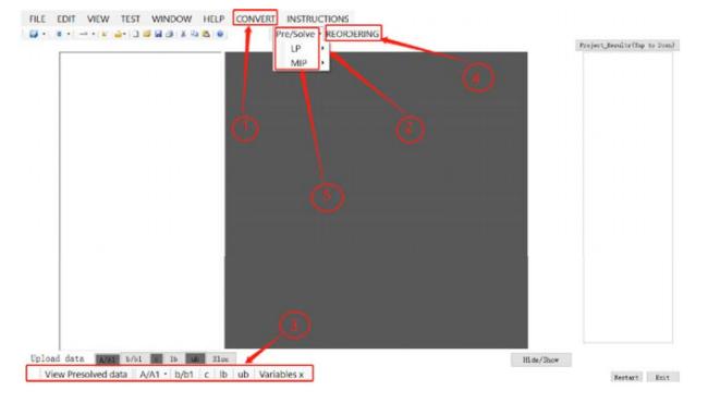
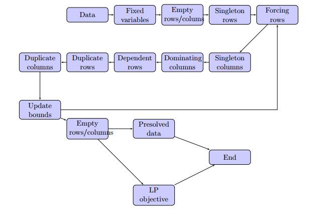
Figure 1 Software home page/screen

Figure 2 Main functionalities

Figure 3 Detailed preprocessing techniques

3 Preprocessing Techniques

3.1 Fixed Variables

3.2 Empty Rows

3.3 Empty Columns

3.4 Singleton Rows

3.5 Forcing Rows

3.5.1 Define Variables Value

3.5.2 Update Bounds: Minimize Original Variables Range

3.6 Singleton Columns

3.7 Doubleton Equation

3.8 Duplicate Rows

3.9 Duplicate Columns

3.10 Dominating Rows

3.11 Dominating Columns

3.12 Dependent Rows

Table 1 Computational results/LP

Table 2 Computational results/MIP

Table 3 Impact of minimum degree reordering/LP

Table 4 Impact of minimum degree reordering (continued)/MIP

4 Minimum Degree Reordering

5 Algorithm Implementation

6 Computational Results

7 Conclusion

{{custom_sec.title}}

{{custom_sec.title}}

References

{{custom_fnGroup.title_en}}

Footnotes

Acknowledgements

{{custom_ack.title_en}}