The Co-Movements Between Crude Oil Price and Internet Concerns: Causality Analysis in the Frequency Domain

Jingjing LI; Ling TANG; Ling LI

doi:10.21078/JSSI-2020-224-16

PDF(672 KB)

Journal of Systems Science and Information ›› 2020, Vol. 8 ›› Issue (3) : 224-239. DOI: 10.21078/JSSI-2020-224-16

The Co-Movements Between Crude Oil Price and Internet Concerns: Causality Analysis in the Frequency Domain

Author information +

History +

Abstract

With the boom of web technology, Internet concerns (IC) have become emerging drivers of crude oil price. This paper makes the first attempt to measure the frequency-varying co-movements between crude oil price and IC in five domains (i.e., fundamentals, supply-demand, crisis, war and weather) by using the frequency causality test method. Based on the monthly Brent spot price and search volumes (SVs) captured by Google Trends from January 2004 to September 2019, new and complementary insights regarding the co-movements between crude oil price and IC are obtained. 1) The co-movements between crude oil price and the IC of supply-demand, war, and weather support a neutral hypothesis at all frequencies due to the characteristics (low value or volatility) of these IC data. 2) There is a unidirectional causal relationship between crude oil price and the IC of fundamentals, running from the latter to the former at low frequencies (long-term). 3) There is a feedback relationship between crude oil price and the IC of crisis, with the IC of crisis driving crude oil price at medium and low frequencies (mid- and long-term) and crude oil price causing the IC of crisis to change permanently. The conclusions of this paper provide important implications for both oil market economists and investors.

Key words

crude oil price / internet concerns / co-movements / frequency causality test / Google trends

Cite this article

EndNote

Ris (Procite)

Bibtex

Download Citations

Jingjing LI , Ling TANG , Ling LI. The Co-Movements Between Crude Oil Price and Internet Concerns: Causality Analysis in the Frequency Domain. Journal of Systems Science and Information, 2020, 8(3): 224-239 https://doi.org/10.21078/JSSI-2020-224-16

1 Introduction

Crude oil is one of the most important commodities in the world, and its price is impacted by a series of indicators, such as supply-demand, financial crisis, war and weather. For example, like most commodities, crude oil price is basically influenced by supply and demand^{[1, 2]}, which are perceived as the natural market forces that influence crude oil price^[3]. Furthermore, financial crisis is widely regarded as one of the most important economic factors that cause oil price fluctuations, especially for the financial crisis in 2008^{[4, 5]}. Moreover, geopolitics such as war usually structurally change crude oil price through impacting oil supply-demand or speculators' anxiety (or expectations)^[6-8]. Finally, extreme weather events also drive up crude oil price if they are dramatic enough^[9]. For instance, hurricane Katrina in 2005 caused crude oil price to rise ＄3 per barrel, and the flooding of the Mississippi River in 2011 also resulted in the increase of oil price since traders were concerned that the flooding would damage oil refineries^[10].

With the financialization of the crude oil market and the rapid development of search technology, Internet concerns (IC) have become the emerging driver of crude oil price. For one thing, the financialization of the crude oil market over the last decade has changed the behaviour of crude oil price and crude oil price drivers^[11]. Although the aforementioned supply-demand factors continue to play an important role, investors' attention, which was proved to be an emerging index to reflect the psychological changes of investors, may further influence the price fluctuations in oil markets. For another, benefitting from the convenience offered by search technology, investors interested in the crude oil market trend to search for information before making an investment. These search traces are captured and processed by search engines. For example, the Google search engine started to collect search volume (SV) data for any keywords in 2004. The SV can represent investors' attention to any specific topic (or keyword) and the SV for similar keywords can be summed to measure the IC for a specific domain. Therefore, IC, as an important proxy for investors' attention on the Internet, is an emerging and promising driver of crude oil price^[12].

Investigating the co-movements between IC and crude oil price has become a hot topic in recent studies. Li, et al.^[13] presented an early attempt to explore the relationship between IC and crude oil price through a linear Granger causality test method. Using an event study methodology and an autoregression-exponential generalized autoregressive conditional heteroscedastic (AR-GARCH) model, Ji and Guo^[12] investigated the effects of four types of oil-related IC on crude oil price. Guo and Ji^[14] analyzed the impact of short- and long-run IC on crude oil price volatility using co-integration and the modified exponential GARCH (EGARCH) model. Similarly, GARCH models are also used by Afkhami, et al.^[15] to demonstrate the predictive power of IC for crude oil price. Based on the IC and (West Texas Intermediate) WTI crude oil price data, Yao, et al.^[16] employed the structural vector autoregression (SVAR) model to empirically explore the impact of IC on WTI crude oil price from January 2004 to November 2016. Qadan and Nama^[17] used daily SV from Google trends to establish that oil shocks Granger-cause the attention of retail investors and show that a heightened number of searches can predict an increase in crude oil price volatility in the trading days that follow through a linear Granger causality test. On account of the closely co-movement between IC and crude oil price, using IC to promote crude oil price forecasting has become a novel and promising research topic; and recent typical examples can be found in the excellent studies of ^{[8, 18, 19]}.

It is obvious that previous studies usually investigate the co-movements between IC and crude oil price at the original frequency with linear models, such as the linear Granger causality test, SVAR, and GARCH. However, the crude oil market as well as crude oil price have been widely proved to have nonlinear characteristics^{[4, 20]} due to the structural changes caused by certain factors, e.g., significant events and energy policy changes. More importantly, crude oil price has been widely proved to have frequency-varying characteristics^{[1, 4]}, and the direction of causality may vary across different frequencies as well. Thus, focusing on the original frequency only gives a partial picture of the causal relationship between crude oil price and IC. Therefore, in this study, we aim to explore the nonlinear and frequency co-movements between crude oil price and IC.

Taking account of the nonlinear and frequency varying characteristics, we apply the frequency causality test method developed by Breitung and Candelon^[21] to investigate the co-movements between crude oil price and IC. Compared to the linear Granger causality test, the frequency causality test has three advantages. First, the frequency causality test allows the dynamic characteristics of the causal relationship at various frequencies (or different time periods) to be determined. Second, this can identify causal relationships even if the underlying linkages among the variables of interest are nonlinear. Finally, this test delivers robust results in the presence of volatility clusters, which is a common characteristic of data with high frequency^[22]. Using this approach, we analyse the causal nexus between crude oil price and IC at all possible frequencies, i.e.,

ω \in (0, π)

Generally, this paper aims to investigate the co-movements between IC and crude oil price through the frequency causality test method proposed by Breitung and Candelon^[21]. Specifically, we first construct five different types of IC using the SV from Google Trends, i.e., the IC of fundamentals, supply-demand, crisis, war and weather. Then, the frequency varying co-movements between the IC and crude oil price are investigated by applying the frequency causality test. The main contributions of this paper can be summarized as three aspects: 1) We make a first attempt to explore the frequency of co-movements between crude oil price and IC; 2) Compared to previous studies, which mainly focus on linear relationships, we investigate both linear and nonlinear co-movements between crude oil price and IC; and 3) inspired by the frequency varying co-movements results, this paper provides important implications for both oil market economists and investors.

The rest of this paper is organized as follows. Section 2 presents the methodological framework of this paper together with a detailed introduction of the frequency causality test method. Section 3 describes the data samples used in this work. Section 4 summarizes the empirical results and gives further implications for both oil market economists and investors. Finally, Section 5 concludes the work.

2 Methodology

2.1 General Framework

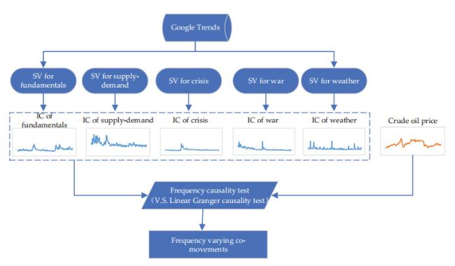
This paper aims to investigate the frequency-varying co-movements between crude oil price and IC with the general framework shown in Figure 1. In particular, two main steps are involved in this framework, i.e., IC construction and the frequency causality test.

Figure 1 The general framework of investigating the frequency co-movements between crude oil price and IC

Full size|PPT slide

In the first step, IC in five domains (i.e., fundamentals, supply-demand, crisis, war and weather) are constructed based on the SV of related keywords collected by Google trends. Fundamentals refer to the fundamental search keywords that may be used by investors when searching online, such as 'crude oil price' and 'crude price'. Since investors sometimes seek information about the drivers of price and not commodities per se ^[15], we also collect the SV regarding the drivers of crude oil price, including supply-demand (keywords of 'oil supply' and 'oil demand'), crisis ('financial crisis' and 'economic crisis'), war ('Libya war' and 'Iraq war'), and weather ('floods' and 'hurricanes'). The SVs for the same types of keywords are summed to yield the corresponding IC in the five domains.

Then, in the second step, the frequency causality test is applied to explore the frequency-varying causal relationship between crude oil price and the IC in the five domains. As for the frequency causality test, the powerful test method proposed by Breitung and Candelon^[21] is adopted in this work. In addition, the traditional linear Granger causality test is also used for comparison.

2.2 Frequency Causality Test

The Granger causality test, first proposed by Granger^[23], aims to test whether the historical information of one time series can help improve the predictability of present and future estimations for another time series. In particular, the Granger causality of two stationary time series,

x_{t}

and

y_{t}

, can be defined as follows. On the one hand, we argue that

y_{t}

does not strictly Granger cause

x_{t}

\Pr (x_{t} | I_{t - 1}) = \Pr (x_{t} | (I_{t - 1} - Y_{t - n}^{n})), t = 1, 2, \dots, T,

(1)

where

\Pr (x_{t} | I_{t - 1})

denotes the conditional probability distribution of series

x_{t}

given the bivariate information set

I_{t - 1} = {X_{t - m}^{m}, Y_{t - n}^{n}}

consisting of an

m

-length lag vector of

x_{t}

and an

n

-length lag vector of

y_{t}

, i.e.,

X_{t - m}^{m} = {x_{t - m}, \dots, x_{t - 1}}

and

Y_{t - n}^{n} = {y_{t - n}, \dots, y_{t - 1}}

. On the other hand, if the equality in Equation (1) is statistically rejected, it can be otherwise proved that the past information of

y_{t}

contributes to the current and future estimations for

x_{t}

, that is,

y_{t}

Granger strictly causes

x_{t}

Although the standard Granger causality test has been one of the most popular econometric techniques to test the causal relationship between two variables, it has some drawbacks. For example, the standard test ignores the possibility that the strength/direction/existence of Granger causality could vary over different frequencies, and the standard test is limited in that it only captures the linear relationship between two variables. To fill the gaps of the standard Granger causality test, Breitung and Candelon^[21] proposed a frequency causality test method that allows for testing for short- and long-term causality between two variables. Compared to the standard test, the frequency causality test has three advantages^[22]: 1) It permits to distinguish the frequency varying characteristics of the causal relationship, either short-run or long-run causality; 2) It can identify causal relationships even if the underlying linkages among the variables of interest are nonlinear; and 3) it delivers robust results in the presence of volatility clusters, a common characteristic of data with high frequency.

In practice, both linear and frequency Granger causality are modelled via the vector autoregression (VAR) model:

θ (L) z_{t} = ε_{t},

(2)

where

z_{t} = [x_{t}, y_{t}]^{'}

is a two-dimensional vector of a time series observed at time

t = 1, 2, \dots, T

;

θ (L) = I - θ_{1} L^{1} - \dots - θ_{p} L^{p}

is a

2 \times 2

lag polynomial, where

L

is a lag operator with

L^{k} z_{t} = z_{t - k}

. The residuals

ε_{t}

, are assumed to be mutually independent and individually have zero mean and constant variance, i.e.,

E (ε_{t}) = 0

E (ε_{t} ε_{t}^{'}) = Σ

, where

Σ

is positive-definite. It should be noted that this model neglects any deterministic terms in Equation (2) for ease of exposition, although in empirical applications, the model typically includes a constant and trend or dummy variables^[21]. Model (2) can be transformed into a matrix form as follows:

θ (L) z_{t} = (\begin{array}{ll} θ_{11} (L) & θ_{12} (L) \\ θ_{21} (L) & θ_{22} (L) \end{array}) (\begin{array}{l} x_{t} \\ y_{t} \end{array}) = ε_{t} .

(3)

Let

G

be a lower triangular matrix and

G^{'}

be an upper triangular matrix of the Cholesky decomposition, with

G^{'} G = Σ^{- 1}

such that

E (η_{t} η_{t}^{'}) = I

and

η_{t} = G ε_{t}

. If the system is assumed to be stationary, we can express the moving average representation of the system as follows:

z_{t} = φ (L) η_{t} = [\begin{array}{ll} φ_{11} (L) & φ_{12} (L) \\ φ_{21} (L) & φ_{22} (L) \end{array}] [\begin{array}{l} η_{1 t} \\ η_{2 t} \end{array}],

(4)

where

φ (L) = θ (L)^{- 1} G^{- 1}

. It was argued by Croux and Reusens^[24] that

y_{t}

are composed of two different parts, i.e., intrinsic parts and predictive parts. The predictive power of

y_{t}

for

x_{t}

can be measured by comparing the predictive parts of the spectrum with the intrinsic parts at each frequency. Then, the testing process for causality running from

y_{t}

x_{t}

at frequency

ω

can be expressed by

M_{y \to x} (ω) = \log [1 + \frac{{| φ_{12} (e^{- i w}) |}^{2}}{{| φ_{11} (e^{- i w}) |}^{2}}] .

(5)

The value of Equation (5) is equal to 0 under the condition that

| φ_{12} (e^{- i w}) | = 0

, which indicates that

y_{t}

does not Granger cause

x_{t}

. In the method of Breitung and Candelon^[21], a necessary and sufficient set of condition for

| φ_{12} (e^{- i w}) | = 0

\sum_{k = 1}^{p} θ_{12, k} \cos (k ω) = 0,

(6)

\sum_{k = 1}^{p} θ_{12, k} \sin (k ω) = 0.

(7)

Since

\sin (k ω) = 0

in the cases of

ω = 0

and

ω = π

, restriction (7) can be dropped in these cases.

In both of the linear and frequency causality test, we need to estimate a VAR model with

p

lags as follows:

x_{t} = α_{11} x_{t - 1} + \dots + α_{1 p} x_{t - p} + β_{11} y_{t - 1} + \dots + β_{1 p} y_{t - p} + ε_{1, t},

(8)

y_{t} = α_{21} y_{t - 1} + \dots + α_{2 p} y_{t - p} + β_{21} x_{t - 1} + \dots + β_{2 p} x_{t - p} + ε_{2, t} .

(9)

When we test whether

y_{t}

Granger causes

x_{t}

, the null hypothesis in the linear Granger causality test is that the coefficients of the lag values of

y_{t}

jointly significantly deviate from zero, i.e.,

H_{0} : β_{11} = β_{12} = \cdot \dots = β_{1 p} = 0

, while in the frequency causality test, the null hypothesis is

H_{0} : R (ω) β_{1} = 0,

(10)

where

β_{1} = {[β_{11}, \dots, β_{1 p}]}^{'}

and

R (ω) = [\begin{array}{llll} \cos (ω) & \cos (2 ω) & \dots & \cos (p ω) \\ \sin (ω) & \sin (2 ω) & \dots & \sin (p ω) \end{array}] .

(11)

Hence, we can test the null hypothesis of no Granger causality at frequency

ω

by employing a standard

F

test for the linear restrictions. The

F

statistic is approximately distributed as

F (2, T - 2 p)

for

ω \in (0, π)

, where the first parameter is the number of restrictions. Otherwise, if we test whether

x_{t}

does not Granger cause

y_{t}

, then the null hypothesis is

H_{0} : R (ω) β_{2} = 0,

(12)

where

β_{2} = [β_{21}, \dots, β_{2 p}]^{'}

. This method can be extended to higher-dimensional systems or to cointegrated VARs^[21].

The frequency causality test has brought new perspectives for co-movements analysis and has therefore been widely applied in a number of areas. For instance, using the frequency causality test, Dergiades, et al.^[22] investigated the co-movements between Google Trends and tourists' arrivals. Bozoklu and Yilanci^[25] applied the frequency causality test to explore the correlation between energy consumption and economic growth for selected organizations from economic cooperation and development (OECD) countries. Gokmenoglu, et al.^[26] explored the causal relationship between economic risk and foreign direct investment (FDI) inflows for the case of Turkey based on the frequency causality test. On account of the advantage in capturing frequency varying co-movements, the frequency causality test is particularly adopted in this paper to investigate the relationship between crude oil price and IC.

3 Data

3.1 IC Construction

To investigate the co-movements between crude oil price and IC, IC in 5 domains, i.e., fundamentals, supply-demand, crisis, war, and weather, are constructed based on the corresponding related SV collected by Google Trends (https://trends.google.com). In addition, considering the different searching behaviours of investors, we choose two search keywords for each domain and sum the SVs of the two related keywords to yield a new index of the IC for further causality analysis. The search keywords of each IC domain are illustrated in Table 1.

Table 1 Search keywords for each IC domain

IC domain	Search keyword
Fundamentals	'crude oil price', 'crude price'
Supply-demand	'oil supply', 'oil demand'
Crisis	'economic crisis', 'financial crisis'
War	'Libya war', 'Iraq war'
Weather	'floods', 'hurricanes'

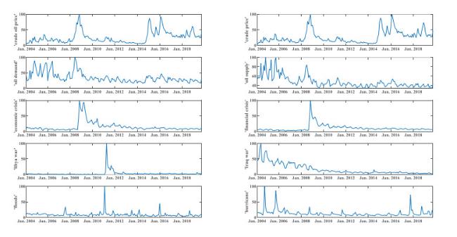
By entering the search keywords into Google trends, the SVs of each keyword are obtained, as shown in Figure 2. In this paper, the monthly SV data and crude oil price ranging from January 2004 to September 2019 are selected. The reason why we choose this data period and frequency is that Google Trends only started to publish the SV in 2004, and Google Trends limits the frequency to monthly data for periods longer than 5 years. In addition, rather than providing the absolute quantity of SV for a keyword, Google Trends normalizes the data between 0 and 100, where 100 is assigned to the date within the interval in which the peak of searching for that keyword is experienced and zero is assigned to dates when the SV for the keyword was less than a certain threshold^[15].

Figure 2 SV for related keywords

Full size|PPT slide

Obviously, the SV for each keyword can well reflect the relevant event that affects crude oil price. For instance, the top values of the SVs for 'economic crisis' and 'financial crisis' appear in October 2008, when the famous global financial crisis burst on a full scale. The financial crisis resulted in sharp price volatility in the crude oil market, and crude oil price suffered severely and dropped to less than ＄30 per barrel in the second half of 2008^[12]. Similarly, the top value of the SV for 'Libya war' appears in March 2011, when the war in Libya broke out. The Libya war resulted in sharp cuts in oil production (by approximately 90%) and therefore an obvious increase in crude oil price. Likewise, the top value of the SV for 'floods' refers to the famous Mississippi floods in the first half year of 2011, and the three peaks of the SV for 'hurricane' correspond to Hurricanes Francis, Rita, Ivan (September 2004), Katrina (September 2005) and Wilma (September 2017). These extreme weather events all led to increases in crude oil price through impacting oil supply-demand or transportation.

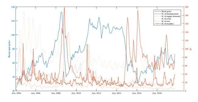
Based on the SVs obtained from Google trends, we construct five IC by summing the SVs of the related keywords in each domain. For example, the SV of the keywords 'crude oil price' and 'crude price' are summed to yield the IC of fundamentals. Figure 3 presents the five constructed IC together with the Brent spot crude oil price collected from U.S. Energy Information Administration (EIA) (https://www.eia.gov). It is obvious that the constructed IC (especially for war and weather) cover more comprehensive information than the separate keywords. For instance, the weather IC experience peak values for the keywords 'hurricanes' and 'floods'. In addition, the 5 constructed IC also exhibit some opposite trends and fluctuations with crude oil price.

Figure 3 The constructed IC and Brent crude oil price

Full size|PPT slide

3.2 Data Statistics

For a further description, Table 2 reports some descriptive statistics for both IC and the Brent crude oil price. One interesting phenomenon is that there is an obvious gap among the volatilities of the various IC, with the IC of fundamentals fluctuating most dramatically (with the largest standard deviation, 39.01) and the IC of weather fluctuating most steadily (with the smallest standard deviation, 14.36).

Table 2 Descriptive statistics of Brent crude oil price and IC

Statistic	Series
Statistic	Brent price	IC of fundamentals	IC of supply-demand	IC of crisis	IC of war	IC of weather
Mean	74.18	52.48	83.04	25.74	19.61	23.2
Median	68.61	41	74	18	11	19
Max.	132.72	198	189	200	110	112
Min.	30.7	7	51	6	3	10
Std. Dev.	26.08	39.01	28.39	25.8	18.59	14.36
Skewness	0.39	1.56	1.69	3.72	2.02	3.79
Kurtosis	1.98	5.3	5.66	19.49	8.13	21.33

Table 3 reports the correlation matrix of crude oil price and IC. It is obvious that all of the constructed IC have a negative relationship with crude oil price, with the IC of fundamentals presenting the maximum correlation (the correlation coefficient is

-

0.35) and the IC of crisis exhibiting the minimum correlation (the correlation coefficient is

-

0.03). The possible reason for these findings is that Google searches mirror investor concerns at least to some extent, thus the concerns will arise when crude oil price declines^[17]. Interestingly, these findings are coincident with the work by Yao, et al.^[16], who proved that investor attention has a significant negative impact on the WTI crude oil price during the sample period.

Table 3 Correlation matrix of Brent crude oil price and IC

	Brent price	IC fundamentals	IC of supply-demand	IC of crisis	IC of war	IC of weather
Brent price	1.00	-0.35	-0.17	-0.03	-0.21	-0.12
IC of fundamentals	-0.35	1.00	0.17	0.27	-0.23	-0.07
IC of supply-demand	-0.17	0.17	1.00	0.03	0.64	0.39
IC of crisis	-0.03	0.27	0.03	1.00	-0.06	-0.09
IC of war	-0.21	-0.23	0.64	-0.06	1	0.31
IC of weather	-0.12	-0.07	0.39	-0.09	0.31	1.00

4 Empirical Results

4.1 Linear Granger Causality Test

Before examining the frequency co-movements between crude oil price and IC, we first explore the traditional linear relationship between them to compare with the results based on the frequency Granger causality test method. In the linear test, we begin with examining the presence of unit root of the data at both the original level and the 1st-difference level. For this purpose, both the augmented Dickey-Fuller (ADF) test and Phillips-Perron test are used to ensure the robustness of the test results, with the results reported in Table 4. Based on the unit root test results, the null hypothesis of a unit root existing is accepted for both the Brent crude oil price and some IC domains (i.e., the IC of supply-demand, crises and fundamentals are detected by the Phillips-Perron test) at the 1% significance level. Therefore, although the null is also rejected for a few IC (i.e., the IC of war and weather), we still apply the 1st-difference data to estimate the VAR models for further linear Granger causality tests.

Table 4 Unit root test for the data

	Original data		1st difference
	ADF test	Phillips-Perron test	ADF test	Phillips-Perron test
Brent price	-2.7	-2.36	-9.20***	-9.10***
IC of fundamentals	-4.14***	-3.70**	-11.95***	-12.73***
IC of supply-demand	-3.08	-3.56**	-12.58***	-12.26***
IC of crisis	-2.71*	-5.60***	-11.96***	-21.51***
IC of war	-6.79***	-6.80***	-13.91***	-34.83***
IC of weather	-9.44***	-9.45***	-9.60***	-55.82***

Notes: *, **, *** denote that the null hypothesis of existing a unit root is rejected at the significance level of 10%, 5%, 1%, respectively.

The linear Granger causality test results between crude oil price and IC are reported in Table 5. In terms of the causality running from IC to the Brent crude oil price, rejection of the null hypothesis is obtained for the IC of fundamentals and crisis at the 5% significance level. The results indicate that the IC of fundamentals and crisis can Granger cause or have predictive power for crude oil price. Furthermore, the results also imply that oil-related fundamental information and economic fluctuations are transmitted quickly through the Internet to oil market investors and that the degree by which market concerns change can influence oil market expectations and thereby influence oil price. Our results are somewhat consistent with the work by Guo and Ji^[14] and Afkhami, et al.^[15]. The former argued that the SV of the fundamental keywords 'Brent crude', 'crude oil' and 'oil price' Granger caused the volatilities of the Brent and WTI crude oil prices, while the latter proved that the IC of fundamentals and crisis were both Granger causes of crude oil price changes. However, in terms of the IC of war, our results present a conclusion different from that of Guo and Ji^[14], who proved that the SV of the keyword 'Libya war' Granger caused a crude oil price change. Our results, however, prove that the IC of war cannot Granger cause a Brent crude oil price change. The hidden reason for these different results may be attributed to the different data samples applied in this paper and Guo and Ji^[14]. In particular, Guo and Ji applied the long-time daily concerns (LTDC) transformed from the SV from Google Trends, while we adopted the original SV, which contains more original and unbroken information.

Table 5 Linear causality between Brent price and IC

IC domains	Lag	H0: IC does not cause Brent		H0: Brent does not cause IC		Results
IC domains	Lag	$χ^{2}$	p-value	$χ^{2}$	p-value	Results
IC of fundamentals	2	7.44	0.02	3.61	0.17	IC $\to$ Brent
IC of supply-demand	5	0.63	0.99	5.49	0.36	$\times$
IC of crisis	2	14.21	0.00	4.88	0.09	IC $\to$ Brent
IC of war	5	5.08	0.41	0.27	1.00	$\times$
IC of weather	3	0.61	0.89	1.06	0.79	$\times$

In terms of the causality running from the Brent crude oil price to IC, all of the linear results adopt the null hypothesis that the Brent price does not Granger cause IC at the significance level of 5%. In other words, the results confirm that the relationships between the Brent crude oil price and IC are unidirectional. IC exhibit useful information for crude oil price forecasting, but not vice versa.

4.2 Frequency Causality Test

The B&C Granger causality test is specially conducted to investigate short-term, mid-term, and long-term relationships between crude oil price and IC in five domains. In particular, the B&C Granger causality test examines causality at all frequencies ranging from 0 to

π

. For a clear illustration, we define

ω \in (0, 0.5]

(periods longer than 12.5 months (almost 1 year)) as long-term,

ω \in (0.5, 2.5]

(periods between 2.5 to 12.5 months) as mid-term and

ω \in (2.5, π]

(periods shorter than 2.5 months) as short-term. Working within the frequency domain can help to disclose causal relationships that may not be distinguishable in the time domain detected by the standard linear causality test.

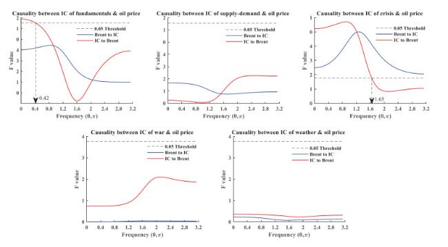
Figure 4 presents the results of the B&C Granger causality test between the IC and Brent crude oil price. It is obvious that the causality changes with frequency (or time period). More precisely, three interesting conclusions can be summarized from these results. First, the causality between crude oil price and the IC of fundamentals supports a unidirectional hypothesis, i.e., there is a unidirectional correlation running from the IC of fundamentals to crude oil price at a significance level of 5%. In addition, the causality relationship is only verified in the low-frequency components

ω \in (0, 4.2)

, indicating that the information of the IC of fundamentals can only promote crude oil price forecasting in the long-term (larger than 15 months). Second, a bidirectional hypothesis is observed between the IC of crisis and crude oil price. On one hand, we found evidence that the IC of crisis causes crude oil price changes in the mid- and long-term (i.e.,

ω \in (0, 1.65)

, periods longer than 3.8 months). In other words, the predictive power of the IC of crisis for crude oil price is confirmed for periods longer than 3.8 months. On the other hand, we also find evidence indicates that crude oil price causes the IC of crisis at any frequency between 0 and

π

. This result confirms a feedback relationship between crude oil price and investors' attention to financial crisis. Third, although supply-demand, war and extreme weather have been widely proven to have significant impacts on crude oil price, their IC, however, have all been proven to exhibit neutral relationships with crude oil price, i.e., there is no Granger causality relationship in either direction.

Figure 4 B&C Granger causality test per IC

Full size|PPT slide

Strangely, the IC of supply-demand, war and weather have all been proven to have a neutral relationship with crude oil price, while they are important drivers of crude oil price. The hidden reasons may lie in the data characteristic of the IC, in particular, the average value and amplitude of the IC data. For example, regarding the IC of supply-demand, the SV value for 'oil supply' is at a low level (with an average value of 10¹) compared to the SV for 'economic crisis' (with an average value of 13) and 'crude oil price' (with an average value of 26). In addition, investors seem to search less for oil supply-demand information online, even in 2014, when the oil price decreased sharply owing to the imbalance between oil supply and demand (as shown in Figure 3). Focusing on the IC of war and weather, the amplitude of the two indexes are both at a low level, as presented in Figure 3 and Table 2. The standard deviations of the IC of war and weather are 18.59 and 14.36, which are much lower than the other IC and the Brent crude oil price. Therefore, the low amplitude of fluctuations of the IC of war and weather lead to their low ability to describe the highly fluctuating oil price. In addition, compared to fundamentals and financial crisis, wars and extreme weather all last for a relative short time or draw short-term public attention, which leads to a large number of low values appearing in the corresponding IC time series (as shown in Figure 3). Thus, the low and stable values cannot capture the rapid changes in oil price.

¹It is worth noting that the average value is obtained here by using the comparison function provided by Google Trends (by comparing the actual SVs for the three keywords) instead of the average of SV shown in Figure 2 because each SV is normalized to between 0 and 100 within the selected time period in Figure 2.

4.3 Summary and Implications

To highlight the advantages of the frequency causality test, we summarize and compare the casual relationship results between crude oil price and the IC obtained from both the standard linear and B&C frequency causality test in Table 6.

Table 6 Summarization and comparation between linear and frequency causality test

IC domain	Linear Granger causality test	Frequency causality test
IC of fundamentals	IC $\to$ Brent	IC $\to$ Brent $\in$ (0, 0.42)
IC of supply-demand	$\times$	$\times$
IC of crisis	IC $\to$ Brent	IC $\to$ Brent $ω$ $\in$ (0, 1.65)), Brent $\to$ IC
IC of war	$\times$	$\times$
IC of weather	$\times$	$\times$

On one hand, our findings from the B&C test are qualitatively similar to those from the linear Granger causality test, at least to some extent. For instance, both the linear and frequency causality test results support a neutral hypothesis between crude oil price and the IC of supply-demand, war and weather. Moreover, the causality running from the IC of fundamentals and crisis to crude oil price is proven to be significant by both the linear and frequency causality test results. On the other hand, more unique results can be captured by the B&C test than the standard linear Granger causality test. For example, the B&C test results suggest that the causality running from the IC of fundamentals and crisis to crude oil price, which is also detected by the standard linear test, is not valid for all frequencies. The causality is only valid at low frequencies ranging from 0 to 0.42 (long-term) for the IC of fundamentals and low and medium frequencies ranging from 0 to 1.65 (mid- and long-term) for the IC of crisis. In addition, contrary to the standard linear test, we further detect the causality running from crude oil price to the IC of crisis by applying the B&C test. The reasons behind this difference may be the advantage of the B&C test in capturing causal relationships even if the underlying linkage among the variables of interest is nonlinear.

The frequency causality test results in this paper have important implications for both oil market economists and investors. Regarding oil market economists, they must take into account possible changing causalities in oil price forecasting. First, the acceptance of the neutral hypothesis between crude oil price and the IC of supply-demand, war and weather demonstrates that the IC in these three domains exhibit no predictive power for crude oil price. Second, the unidirectional causality running from the IC of fundamentals at low frequencies (lower than 0.42) indicates that the IC of fundamentals can promote crude oil price forecasting in the long-term (longer than 15 months). Third, the existence of the causality running from the IC of crisis to crude oil price at medium and low frequencies (lower than 1.65) suggests that the IC of crisis has predictive power for crude oil price over the mid- and long-term (longer than 3.8 months). Therefore, compared to most existing studies that apply IC for crude oil price forecasting directly without detecting their frequency co-movements, we can offer important insights for using appropriate IC for crude oil price forecasting in different time periods. Regarding oil market investors, they should pay attention to specific IC changes and make dynamic decisions accordingly. For one thing, investors should be conscious of the empirical results that not all IC can Granger cause oil price fluctuations. For example, our results only confirm that the IC of fundamentals and crisis can Granger affect crude oil price temporally. In this regard, oil market investors should place particular emphasis on the impact of these two important IC on crude oil price fluctuations. Additionally, investors must take into account changing causalities and make investment decisions accordingly. For example, investors can use the IC of fundamentals for long-term investment and the IC of crisis for mid- and long-term investment. Overall, oil market investors should take into consideration not only the causality direction between IC and crude oil price but also whether the direction is temporal or permanent, in other words, whether it changes due to the time period.

5 Conclusions

With the financialization of the crude oil market, informatization and networking have become new characteristics of the oil market. In particular, investors' concerns and preferences can be quickly transmitted to the oil market through the Internet. Therefore, as a typical index for investors' concerns, IC has become an emerging driver of crude oil price. More importantly, understanding the co-movements of IC and crude oil price may have important implications for oil market economists and investors. Thus, this paper aims to investigate the co-movements between IC and crude oil price through the frequency causality test method. Different from existing studies, which only pay attention to linear and original correlations, our work is the first that focuses on the frequency-varying co-movements between crude oil price and IC. Specifically, we employ a two-step process to estimate the co-movements. In the first step, we construct five different types of IC from the SV captured by Google Trends, i.e., the IC of fundamentals, supply-demand, crisis, war and weather. In the second step, the frequency varying co-movements among the five IC and crude oil price are investigated based on the frequency causality test proposed by Breitung and Candelon^[21]. For comparison, the standard linear Granger causality test is also used to detect the general and linear causal relationship between crude oil price and IC.

Choosing the monthly Brent spot price and the SV collected from Google Trends as data samples, we find that the casual co-movements between crude oil price and IC generally change with frequency and that the B&C test can capture more information compared with the linear Granger causality test. More precisely, three main conclusions are drawn from the frequency causality test. First, the co-movements between crude oil price and the IC of supply-demand, war and weather support a neutral hypothesis (i.e., no causal relationship) at all frequencies. The reason for this result may lie in the data characteristic of the three IC, particularly the low value of the IC of supply-demand and the low amplitude of the IC of war and weather. Second, the feedback hypothesis is valid between crude oil price and the IC of crisis, where the IC of crisis drives crude oil price at medium and low frequencies (mid- and long-term) and crude oil price causes the IC of crisis to change permanently. Third, a unidirectional causality relationship is suggested between crude oil price and the IC of fundamentals, running from the IC of fundamentals to crude oil price at low frequencies (long-term).

Our results have several implications for both oil market economists and investors. Regarding oil market economists, they must take into account possible changing causalities in oil price forecasting. In particular, our results supply important insights for using appropriate IC for crude oil price forecasting in different time periods. Regarding oil market investors, they must consider the changing causalities and make investment decisions accordingly. In this regard, oil market investors should take into consideration not only the causality direction between IC and crude oil price but also whether the direction is temporal or permanent, in other words, whether it changes due to the time dimension.

This research provides a new perspective on investigating the frequency varying co-movements between crude oil price and IC. One possible extension of this research is constructing better proxies of IC, such as collecting more keywords in more domains. Another possible extension of this research is investigating the potential asymmetries in the causal effects between crude oil price and IC. In this case, decomposing the total volatility into good and bad volatility allows one to check whether the uncertainty arising from positive changes in oil prices and IC is propagated differently than the uncertainty due to negative changes in oil prices and IC. We will look into these issues in the near future.

References

Publishing order | Descend order by publishing year | Descend order by cited within

1	Yu L A, Wang S Y, Lai K K. Forecasting crude oil price with an EMD-based neural network ensemble learning paradigm. Energy Economics, 2008, 30 (5): 2623- 2635. https://doi.org/10.1016/j.eneco.2008.05.003 Cited in this article [2]

2	Yin X, Peng J, Tang T. Improving the forecasting accuracy of crude oil prices. Sustainability, 2018, 10 (2): 454. https://doi.org/10.3390/su10020454 Cited in this article [1]

3	Wang Y D, Liu L. Is WTI crude oil market becoming weakly efficient over time? New evidence from multiscale analysis based on detrended fluctuation analysis. Energy Economics, 2010, 32 (5): 987- 992. https://doi.org/10.1016/j.eneco.2009.12.001 Cited in this article [1]

4	Yu L, Li J, Tang L, et al. Linear and nonlinear Granger causality investigation between carbon market and crude oil market: A multi-scale approach. Energy Economics, 2015, 51, 300- 311. https://doi.org/10.1016/j.eneco.2015.07.005 Cited in this article [3]

5	Lu Y, Yang L, Liu L. Volatility spillovers between crude oil and agricultural commodity markets since the financial crisis. Sustainability, 2019, 11 (2): 396. https://doi.org/10.3390/su11020396 Cited in this article [1]

6	Su X, Zhu H, Yang X. Heterogeneous causal relationships between spot and futures oil Prices: Evidence from quantile causality analysis. Sustainability, 2019, 11 (5): 1359. https://doi.org/10.3390/su11051359 Cited in this article [1]

7	Noguera-Santaella J. Geopolitics and the oil price. Economic Modelling, 2016, 52, 301- 309. https://doi.org/10.1016/j.econmod.2015.08.018

8	Wang J, Athanasopoulos G, Hyndman R J, et al. Crude oil price forecasting based on internet concern using an extreme learning machine. International Journal of Forecasting, 2018, 34 (4): 665- 677. https://doi.org/10.1016/j.ijforecast.2018.03.009 Cited in this article [2]

9	Cruz A M, Krausmann E. Vulnerability of the oil and gas sector to climate change and extreme weather events. Climatic Change, 2013, 121 (1): 41- 53. https://doi.org/10.1007/s10584-013-0891-4 Cited in this article [1]

10	Lai A, Song L, Peng Y, et al. Exploring crude oil impacts to oil stocks through graphical computational correlation analysis. International Conference on Neural Information Processing. Springer-Verlag, 2012. Cited in this article [1]

11	Lammerding M, Stephan P, Trede M, et al. Speculative bubbles in recent oil price dynamics: Evidence from a Bayesian Markov-switching state-space approach. Energy Economics, 2013, 36, 491- 502. https://doi.org/10.1016/j.eneco.2012.10.006 Cited in this article [1]

12	Ji Q, Guo J F. Oil price volatility and oil-related events: An Internet concern study perspective. Applied Energy, 2015, 137, 256- 264. https://doi.org/10.1016/j.apenergy.2014.10.002 Cited in this article [3]

13	Li X, Ma J, Wang S Y, et al. How does Google search affect trader positions and crude oil prices?. Economic Modelling, 2015, 49, 162- 171. https://doi.org/10.1016/j.econmod.2015.04.005 Cited in this article [1]

14	Guo J F, Ji Q. How does market concern derived from the Internet affect oil prices?. Applied Energy, 2013, 112, 1536- 1543. https://doi.org/10.1016/j.apenergy.2013.03.027 Cited in this article [4]

15	Afkhami M, Cormack L, Ghoddusi H. Google search keywords that best predict energy price volatility. Energy Economics, 2017, 67, 17- 27. https://doi.org/10.1016/j.eneco.2017.07.014 Cited in this article [4]

16	Yao T, Zhang Y J, Ma C Q. How does investor attention affect international crude oil prices?. Applied Energy, 2017, 205, 336- 344. https://doi.org/10.1016/j.apenergy.2017.07.131 Cited in this article [2]

17	Qadan M, Nama H. Investor sentiment and the price of oil. Energy Economics, 2018, 69, 42- 58. https://doi.org/10.1016/j.eneco.2017.10.035 Cited in this article [2]

18	Han L Y, Lv Q N, Yin L B. Can investor attention predict oil prices?. Energy Economics, 2017, 66, 547- 558. https://doi.org/10.1016/j.eneco.2017.04.018 Cited in this article [1]

19	Elshendy M, Colladon A F, Battistoni E, et al. Using four different online media sources to forecast the crude oil price. Journal of Information Science, 2018, 44 (3): 408- 421. https://doi.org/10.1177/0165551517698298 Cited in this article [1]

20	Lin E B, Liang C C, Tsai W. Nonlinear relationships between oil prices and implied volatilities: Providing more valuable information. Sustainability, 2019, 11 (14): 3906. https://doi.org/10.3390/su11143906 Cited in this article [1]

21	Breitung J, Candelon B. Testing for short- and long-run causality: A frequency-domain approach. Journal of Econometrics, 2006, 132 (2): 363- 378. https://doi.org/10.1016/j.jeconom.2005.02.004 Cited in this article [8]

22	Dergiades T, Mavragani E, Pan B. Google trends and tourists' arrivals: Emerging biases and proposed corrections. Tourism Management, 2018, 66, 108- 120. https://doi.org/10.1016/j.tourman.2017.10.014 Cited in this article [3]

23	Granger C W. Investigating causal relations by econometric models and cross-spectral methods. Econometrica: Journal of the Econometric Society, 1969, 424- 438. Cited in this article [1]

24	Croux C, Reusens P. Do stock prices contain predictive power for the future economic activity? A Granger causality analysis in the frequency domain. Journal of Macroeconomics, 2013, 35, 93- 103. https://doi.org/10.1016/j.jmacro.2012.10.001 Cited in this article [1]

25	Bozoklu S, Yilanci V. Energy consumption and economic growth for selected OECD countries: Further evidence from the Granger causality test in the frequency domain. Energy Policy, 2013, 63, 877- 881. https://doi.org/10.1016/j.enpol.2013.09.037 Cited in this article [1]

Gokmenoglu K, Kirikkaleli D, Eren B M. Time and frequency domain causality testing: The causal linkage between FDI and economic risk for the case of Turkey. Journal of International Trade and Economic Development, 2019, 28 (6): 649- 667.

https://doi.org/10.1080/09638199.2018.1561745

Cited in this article [1]

Funding

National Fund of Philosophy and Social Science of China(18ZDA106)

PDF(672 KB)

213

Accesses

Citation

Detail

Sections

Recommended

Abstract
Key words
Cite this article
1 Introduction
2 Methodology
2.1 General Framework
Figure 1 The general framework of investigating the frequency co-movements between crude oil price and IC
2.2 Frequency Causality Test
3 Data
3.1 IC Construction
Table 1 Search keywords for each IC domain
Figure 2 SV for related keywords
Figure 3 The constructed IC and Brent crude oil price
3.2 Data Statistics
Table 2 Descriptive statistics of Brent crude oil price and IC
Table 3 Correlation matrix of Brent crude oil price and IC
4 Empirical Results
4.1 Linear Granger Causality Test
Table 4 Unit root test for the data
Table 5 Linear causality between Brent price and IC
4.2 Frequency Causality Test
Figure 4 B&C Granger causality test per IC
4.3 Summary and Implications
Table 6 Summarization and comparation between linear and frequency causality test
5 Conclusions
References
Funding

Received	Accepted	Published
2020-03-30	2020-05-16	2020-06-25
Issue Date
2020-06-25

Please choose a citation manager

Content to export

Abstract

Key words

Cite this article

1 Introduction

2 Methodology

2.1 General Framework

Figure 1 The general framework of investigating the frequency co-movements between crude oil price and IC

2.2 Frequency Causality Test

3 Data

3.1 IC Construction

Table 1 Search keywords for each IC domain

Figure 2 SV for related keywords

Figure 3 The constructed IC and Brent crude oil price

3.2 Data Statistics

Table 2 Descriptive statistics of Brent crude oil price and IC

Table 3 Correlation matrix of Brent crude oil price and IC

4 Empirical Results

4.1 Linear Granger Causality Test

Table 4 Unit root test for the data

Table 5 Linear causality between Brent price and IC

4.2 Frequency Causality Test

Figure 4 B&C Granger causality test per IC

4.3 Summary and Implications

Table 6 Summarization and comparation between linear and frequency causality test

5 Conclusions

{{custom_sec.title}}

{{custom_sec.title}}

References

{{custom_fnGroup.title_en}}

Footnotes

Funding

Share

模态框（Modal）标题

Please choose a citation manager

Content to export

Abstract

Key words

Cite this article

1 Introduction

2 Methodology

2.1 General Framework

Figure 1 The general framework of investigating the frequency co-movements between crude oil price and IC

2.2 Frequency Causality Test

3 Data

3.1 IC Construction

Table 1 Search keywords for each IC domain

Figure 2 SV for related keywords

Figure 3 The constructed IC and Brent crude oil price

3.2 Data Statistics

Table 2 Descriptive statistics of Brent crude oil price and IC

Table 3 Correlation matrix of Brent crude oil price and IC

4 Empirical Results

4.1 Linear Granger Causality Test

Table 4 Unit root test for the data

Table 5 Linear causality between Brent price and IC

4.2 Frequency Causality Test

Figure 4 B&C Granger causality test per IC

4.3 Summary and Implications

Table 6 Summarization and comparation between linear and frequency causality test

5 Conclusions

{{custom_sec.title}}

{{custom_sec.title}}

References

{{custom_fnGroup.title_en}}

Footnotes

Funding