1 Introduction
The emergence of economic globalization and financial integration has brought global financial markets closer together, and accelerated spread and transmission of crises and risks among financial markets. The rapid development of financial market makes its internal relationship more and more complex. Correlation is an important part of quantitative analysis of financial market related structure, and it is also a central issue in financial risk analysis.
In the traditional risk management, Pearson correlation coefficient method and Granger causality analysis method are used to describe and measure the correlation between sequences, but these methods have some drawbacks and limitations. For example, the Pearson correlation coefficient between sequences can only measure linear correlation and requires a limited variance. However, most of yields sequences of financial assets presented with fat tails, variance may not exist, so Pearson correlation coefficients can not be used to reflect the relevance of such data. Furthermore, Pearson correlation coefficient can only describe correlation pattern between sequences, but can not capture relevant features of tails of sequences. And the Pearson correlation coefficient method usually needs to assume that joint distribution obeys normal distribution or distribution, and requires each marginal distribution function to be of the same type. But such assumptions may not be true in many cases.
Calculating a correlation analysis, we need to know density function of joint distribution of sequences. When using Copula
[1] to construct joint distribution, the joint distribution is not only subject to the constraint that marginal distribution belongs to same distribution type, but also distribution function of single sequence and dependent structure between sequences can be studied separately, so the application of Copula is more flexible. Since Embrachts
[2] introduced Copula into financial risk management, it has become a powerful research tool in this field because of its special advantages in analyzing relevance. Many scholars have also made many meaningful contributions in this field. Durrleman
[3] gave a few methods for choice of Copulas in financial modeling, Li
[4] applied Copula function method to study of default correlation, Jaworski
[5] gave a comprehensive introduction to the theory and application of Copula, Rodriguez
[6] used the Copula method to measure financial contagion, Huang
[7] estimated the risk value of portfolio using conditional Copula-GARCH method, Aloui
[8] studied the conditional dependence structure of oil price and exchange rate by Copula-GARCH method, Kim
[9] analyzed direction dependence based on asymmetric Copula regression model, Jondeau
[10] applied the condition-dependent Copula-GARCH model to international stock market research, many follow-up scholars have carried out more in-depth research and application.
Since Hu
[11] first proposed a mixture Copula(M-Copula) model in his article, M-Copula has more comprehensive reflection of correlation between sequences, because M-Copula combines advantages of each single Copula in its components. Therefore, M-Copula has attracted attention of many researchers. Ouyang
[12] studied the dependence based on M-Copula model and its application in the risk management, Ignatieva
[13] analyzed the Australian electricity market spot price dependent model and risk management applications with M-Copula, Harb
[14] uses M-Copula to price CDS spread adjusted by credit valuation.
The parameters of Copula model can be estimated by traditional methods such as moment estimation and maximum likelihood estimation. Shih
[15] deduced the correlation parameters of copula model for binary survival data, Chen
[16] estimates the semi-parametric time series model based on Copula, Joe
[17] studied the asymptotic efficiency of two-stage estimation method based on the Copula model. However, M-Copula model is complex in structure and usually has no analytic solutions by using likelihood method. In recent years, some scholars have used optimization algorithms to estimate the parameters of M-Copula model. Liu
[18] improved and tested the maximum likelihood estimation iteration (fixed point) algorithm based on Copula model, Zhang
[19] used a conventional expectation maximization algorithm to estimate the parameters of the mixed connection function effectively.
Based on the inspiration of the previous article, this paper will be based on the M-Copula-EGARCH-M-GED model analysis, take Composite index and fund index of Shanghai Stock Exchange as an example to analyze the correlation between Shanghai Stock Exchange and fund market. The parameters of the M-Copula model are estimated by EM algorithm.
2 Establishment of Model
2.1 Correlation Theory of Copula Function
Theorem 1 Sklar's theorem , see [
20])
Let H be a joint distribution function with margins F and G. Then there exists a copula C such that for all .
If and are continuous, then is unique; otherwise, is uniquely determined on. Conversely, if is a Copula and and are distribution function, then the function defined by Equation (1) is a joint distribution function with margins and .
Sklar's theorem reveals the role of Copula function in linking joint distribution and marginal distribution, which lays a theoretical foundation for the application of Copula function in financial analysis.
M-Copula is a linear convex combination of Copula functions, which is more flexible than single Copula function. Because it combines the advantages of component Copula, it can simultaneously display the ability of each Copula to describe different related features of sequence. So as to enhance its strengths and avoid its weaknesses, and achieve better results in capturing more complex related features. The general form of the M-Copula model is as follows in Equation (2), if , , , are Copula functions, then their convex combination
also a Copula function, where is the weight parameter, is the relevant parameter.
In the third section of empirical study, by analyzing the selected data, select Gumbel, Clayton, and Frank function in Archimedes Copula, and the M-Copula model by linear combination equation (3), the correlation between two yields sequence is studied and compared.
in which , , represents the weight of each Gumbel, Clayton and Frank function weighting coefficients, also is the function M-Copula weight parameter (, , ).
2.2 Copula-EGARCH-M-GED Model
Copula model building process, select an appropriate marginal distribution is a key step. Most of the conditional distributions of financial time series have the characteristics of time-varying fluctuations, clustering, skewness, spikes and fat tails. The ARCH model can characterize these properties, and thus can better describe condition distribution of financial yields sequences, which is conducive to improving the accuracy of Copula model, so as to achieve better modeling results.
The conditional distribution of financial time series often has the characteristics of sharp peaks and fat tails. The fat tail characteristics of
distribution and GED distribution (generalized error distribution) perform well when characterizing the above characteristics of data. The GARCH model has a strong generalization ability, and the ability to describe time series volatility is better than the ARCH model. The exponential GARCH (EGARCH) model proposed by Nelson
[21] overcomes the non-negative limitation of parameters in the linear GARCH(LGARCH) model, and overcomes the shortcomings of the LGARCH model that it is difficult to judge persistence of the conditional variance fluctuation source. The GARCH-M model was proposed by Engle
[22], it is the fact that the GARCH model takes into account the fact that the conditional variance changes with time. The GARCH model is extended so that the conditional variance can directly affect the mean of the returns. The economic significance of the GRACH-M model is very obvious and has been widely recognized. Therefore, the EGARCH-M-GED model is used to fit the sample yield sequence. The binary Copula-EGARCH(1, 1)-M-GED form is as follows:
The standard deviations of the marginal distribution functions are respectively the thickness parameters of the tail are respectively and , and the shape parameters are respectively and
2.3 Expectation Maximization Algorithm
EM algorithm (expectation maximization algorithm) is not only an iterative optimization strategy, but also a data addition algorithm. In 1977, EM algorithm was summarized by Dempster
[23] for maximum likelihood estimation or maximum posterior probability estimation of parameters of probability model with latent variables. The most commonly used method to obtain the estimation of model parameters from sample observation sequence is to maximize logarithmic likelihood function of model distribution. However, in some cases, the observed data has unobserved hidden variables, and the estimated results of model parameters cannot be directly obtained by maximizing log-likelihood function. In this case, the EM algorithm can be considered. Each iteration of the EM algorithm consists of two steps: Expectations are computed in step E and maximization of likelihood functions in step M. The hidden variables and model parameters are iteratively updated until the convergence, the estimated results of model parameters can be obtained.
In the empirical research, the yield series where its joint distribution function is formula (3) M-Copula. That is
Parameters , Estimated by EM algorithm. In order to discuss concisely, is recorded as and as and respectively.
Implicit variables are introduced to obtain logarithmic likelihood functions for complete data: The probability distribution model of yield series is the model equation (3), but it is unknown which sub-model a pair of belongs to. Therefore, variable is introduced to reflect the sub-model of yield series , which is defined as follows:
The yield series is known, and after adding the unobserved data , the complete data is
The likelihood function of complete data is obtained:
the .
Thus, the logarithmic likelihood function of complete data is
Step E Computing expectations for logarithmic likelihood function of complete data with respect to implicit variable , under the condition that and the parameter are known by the estimation. It is recorded as a Q function.
Calculate and mark
denotes the probability that the first i-pair sequence belongs to the sub-model k, so it is called the response of the sub-model k to the yield sequence
The substitution Formula (2.7) is available.
Step M Calculate the maximum value of function to The model parameters of iteration in the new round are as follows
is used to represent the parameters of
The results are as follows:
The E-step and M-step are iterated repeatedly until convergence, and finally the estimation results of parameters are obtained.
2.4 Testing Copula Model
Copula goodness-of-fit test is the criterion to judge and measure the excellent modeling effect of Copula model, Berg
[24] summarized and compares several methods of Copula goodness of fit test. In this paper, two methods are used to test the copula model.
Distance criterion The empirical distribution function is used as the simulation value of the real Copula function, comparison of the estimated Copula function and real function Copula distance . The square Euclidean distance between Copula function and empirical Copula function is defined as:
The smaller the value of is, the better the fitting effect will be.
Statistical Mis a distribution-dependence test statistic introduced by Hu
[11]. It is used to evaluate the goodness of fit Copula function. It is based on the probabilistic integral transformation of the observation sequence
and
to obtain a new uniform sequence
and
and to construct a table
containing
cells. The cella in row
and column
in the table are denoted as
. For any point
if
and
, then
represents a set of probability whose lower bound is
and upper bound is
denotes the number of actual observation points in cell
denotes the number of points in cell
predicted by Copula model. The
-test statistic M, which evaluates the goodness of fit of Copula function, is expressed as:
Statistical M obeys distribution with degree of freedom . In this paper, is selected according to the total number of observation points.
3 Empirical Analysis
3.1 Descriptive Statistical Analysis of Sample Data
This paper selects the Shanghai Composite Index (SHCI) and the fund index (SHFI) issued by the Shanghai Stock Exchange in China's financial market to represent the stock and fund markets for correlation analysis. Taking the daily closing price as a sample, the price is taken as the index closing price on the day day, and the yield is defined as . The selected data period is from January 4, 2013 to October 11, 2018, with a total of 1402 observations.
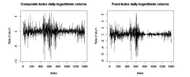
Time series
Figure 1 and descriptive statistical results
Table 1 shows that logarithmic yields sequences of composite index and fund index have the characteristics of general financial time series with fluctuation clusters, spikes and fat tails. Moreover, the test results of the normality test JB statistic
[25] indicate that normal distribution hypothesis is rejected.
Figure 1 Time series diagram of logarithmic return rate |
Full size|PPT slide
Table 1 Descriptive statistical results |
| index | Max | Min | Mean | std.Dev | Skewness | Kurtosis | JB |
| SHCI | 6.3329 | 9.4791 | 0.0133 | 1.4799 | 0.7340 | 6.6969 | 2755 |
| SHFI | 6.5422 | 7.5514 | 0.0247 | 1.0434 | 0.8390 | 11.0702 | 7344.6 |
3.2 Time Series Analysis and Modeling
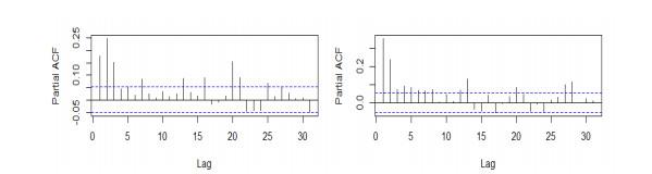
The ACF graph of the two logarithmic rate of return series in Figure 2 shows that there is basically no autocorrelation. The PACF plot of the square of the logarithmic return series in Figure 3 shows that there is a significant autocorrelation in the high-order lag period. And the value of the Ljung-Box test of the square of the two return series is small , so there is obvious ARCH effect.
Figure 2 ACF of logarithmic return series of composite index (left) and fund index (right) |
Full size|PPT slide
Figure 3 PACF of the square of logarithmic return series of composite index and fund index |
Full size|PPT slide
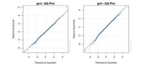
The sample data was fitted using the EGARCH(1, 1)-M-GED model. The Q-Q diagram of the fitting results is shown in Figure 4. It can be seen that the EGARCH(1, 1)-M-GED model has a good fitting effect on the selected samples.
Figure 4 Q-Q graph of EGARCH-M-GED fitting results for logarithmic return series of composite index and fund index |
Full size|PPT slide
The edge distribution of the return series is modeled by EGARCH(1, 1)-M-GED, and Tables 2 and 3 are the estimation and test results.
Table 2 Parameter estimation table of shanghai composite index return sequence |
| Parameter | Estimate | std.Error | value | |
| 0.0245 | 0.0127 | 1.9216 | 0.0547 |
| 0.0179 | 0.0118 | 1.5137 | 0.1301 |
| 0.0022 | 0.0030 | 0.7126 | 0.4761 |
| 0.0105 | 0.0147 | 0.7115 | 0.4768 |
| 0.1431 | 0.0091 | 15.70 | 0.0000 |
| 0.9933 | 0.0000 | 463290 | 0.0000 |
| 1.0812 | 0.0513 | 21.08 | 0.0000 |
Table 3 Parameter estimation table of ShangHai fun index return sequence |
| Parameter | Estimate | std.Error | value | |
| 0.0145 | 0.0023 | 6.2501 | 0.0000 |
| 0.0014 | 0.0023 | 0.5818 | 0.5607 |
| 0.0049 | 0.0053 | 0.9153 | 0.3600 |
| 0.0035 | 0.0208 | 0.1707 | 0.8645 |
| 0.2608 | 0.0302 | 8.6264 | 0.0000 |
| 0.9939 | 0.0018 | 539.49 | 0.0000 |
| 1.0066 | 0.0497 | 20.26 | 0.0000 |
From Table 2 and Table 3, we know that , which shows that both the Shanghai Stock Market and the fund market have leverage effect; and is greater than 1, which shows that the current information in the model is very important for predicting future conditional variance. It can be seen that the EGARCH(1, 1)-M-GED model has a good effect on the conditional edge distribution of the fitted sequence. Therefore, it is reasonable to select the EGARCH(1, 1)-M-GED model to describe the conditional edge distribution of the sequence.
3.3 Copula Function Modeling
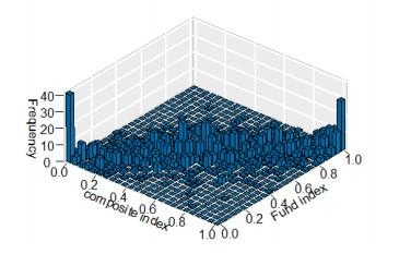
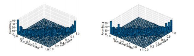
The scatter plot 5 of the empirical distribution after the residual sequence transformation shows that the tail dependence between the two sequences is strong. Given the frequency distribution histogram 6 corresponding to the above samples, the joint distribution of the two sample return series can be observed. The frequency of the sample at the upper and lower tails is higher and asymmetrical, and the distribution of the lower tail is heavier than that of the upper tail. It can be judged that the at the lower end is a non-decreasing function with respect to the variable , and the situation at the upper tail is similar. Therefore, it shows that there is a strong tail correlation at the top and bottom.
Figure 5 Empirical Distribution |
Full size|PPT slide
Figure 6 Frequency distribution histogram |
Full size|PPT slide
A single Gumbel, Clayton and Frank Copula function is selected for modeling analysis. The parameters in the Copula function are estimated by the method of empirical distribution function in nonparametric kernel density estimation.
Tables 4 show that different Copula models have great differences in the ability to describe the correlation between composite index and fund index, the Euclidean distance square of M-Copula is smaller than that of Archimedes Copula in Table 4, and the M-statistics of M-Copula are significant at the level of 0.05, that is to say, the fitting effect of M-Copula is the best. The weight coefficient of the Gumbel function in M-Copula is the largest, and the weight coefficient of Frank and Clayton is small, indicating that there is an asymmetric tail correlation between yields sequence of composite index and fund index. The estimated values of the relevant parameters indicate that there is a strong positive correlation between composite index and fund index.
Table 4 Parameter estimation results of Copula model |
| | Copula | Parameter | Likelihood function | | M |
| | Gumbel | 0.2332 | 1700.56 | 0.5370 | 191.4759(103) |
| | Clayton | 2.0841 | 1550.67 | 0.0631 | 501.3113(122) |
| | Frank | 16.1227 | 1574.97 | 0.1646 | 207.9246(115) |
| Relational | Gumbel | 0.1995 | 1832.18 | 0.0372 | 114.7360*(108) |
| Clayton | 4.6519 |
| Frank | 5.6218 |
| Weight | Gumbel | 0.5693 |
| Clayton | 0.3670 |
| Frank | 0.0637 |
| * The values in parentheses of statistic M are corresponding degrees of freedom, and * is significant at the level of 0.05. |
Figure 7 is a frequency distribution diagram of empirical distribution obtained by probability integral transformation of composite index and fund index yields sequences, and the estimated frequency distribution of probability distribution determined by M-Copula. The M-Copula distribution is very close to the empirical distribution, and most of the observation points fall near the main diagonal of . This indicates that there is a significant positive correlation between composite index and fund index, which is consistent with the results of estimated parameters of M-Copula. In addition, there is an asymmetric tail-related structure between composite index and fund index.
Figure 7 Frequency distribution of empirical distribution and M-Copula probability distribution |
Full size|PPT slide
3.4 Result Analysis
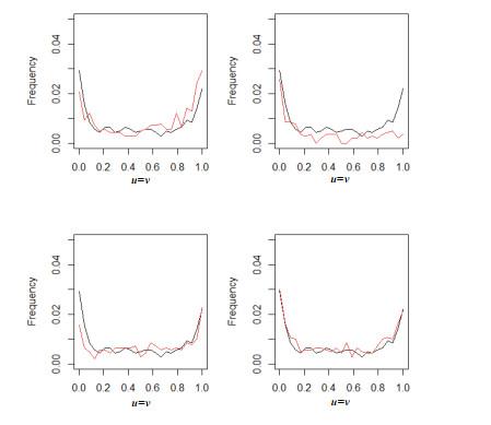
Figure 8 shows a comparison of empirical distribution and frequency distribution of several Copula distributions at . The variation of distribution on the main diagonal of reflects coordinated movement between financial markets. Four kinds of Copula are better characterize the effect of correlation between two yields sequences in normal times. However, there is a big difference in the correlation between two yields sequences when the tail of the distribution, that is, the extreme event occurs. Gumbel underestimates lower tail and overestimates upper tail, and indicates that correlation between upper tail and tail is stronger, which is contrary to higher correlation between lower tail and the tail of the empirical Copula function distribution. Clayton clearly overestimates the bottom and underestimates upper tail. Frank is underestimated for both upper and lower tails and does not reflect the asymmetric tail correlation between composite index and fund index. M-Copula is very close to the empirical distribution at upper and lower tails, and can accurately capture the correlation between two periods of two yields sequences, which can reflect the correlation pattern between two indexes more realistically.
Figure 8 Comparison of Gumbel, Clayton, Frank and M-copula with empirical distribution |
Full size|PPT slide
4 Summary
Although Copula has the property of being able to separate marginal distribution from joint distribution, it provides great convenience in correlation analysis. However, the increasingly complex changes in financial markets make it difficult to accurately describe the relevant structures between markets using single Copula model. In this case, M-Copula is due to its special construction. Combining the characteristics of single Copula model, the form is flexible, and the scope of application is broader, which can portray more complex correlations between financial markets. In this paper, combined with the EGARCH-M-GED model, M-Copula is mainly used to study the correlation between composite index and fund index. A comparative analysis of the correlation between two yields sequences of single Archimedes Copula and M-Copula, the parameters of M-Copula were estimated using EM algorithm. The results of empirical research show that M-Copula can more accurately capture asymmetric tail correlation between two yields sequences.
{{custom_sec.title}}
{{custom_sec.title}}
{{custom_sec.content}}
 PDF(274 KB)

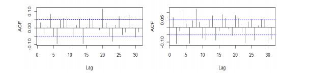
 Figure 1 Time series diagram of logarithmic return rate
 Table 1 Descriptive statistical results


