Bifractional Black-Scholes Model for Pricing European Options and Compound Options

Feng XU

doi:10.21078/JSSI-2020-346-10

PDF(167 KB)

Journal of Systems Science and Information ›› 2020, Vol. 8 ›› Issue (4) : 346-355. DOI: 10.21078/JSSI-2020-346-10

Bifractional Black-Scholes Model for Pricing European Options and Compound Options

Author information +

History +

Abstract

Recent empirical studies show that an underlying asset price process may have the property of long memory. In this paper, it is introduced the bifractional Brownian motion to capture the underlying asset of European options. Moreover, a bifractional Black-Scholes partial differential equation formulation for valuing European options based on Delta hedging strategy is proposed. Using the final condition and the method of variable substitution, the pricing formulas for the European options are derived. Furthermore, applying to risk-neutral principle, we obtain the pricing formulas for the compound options. Finally, the numerical experiments show that the parameter HK has a significant impact on the option value.

Key words

bifractional Brownian motion / compound options / long memory property / pricing model

Cite this article

EndNote

Ris (Procite)

Bibtex

Download Citations

Feng XU. Bifractional Black-Scholes Model for Pricing European Options and Compound Options. Journal of Systems Science and Information, 2020, 8(4): 346-355 https://doi.org/10.21078/JSSI-2020-346-10

1 Introduction

The traditional study of option pricing is based on the assumption that the underlying asset obeys the geometric Brownian motion^[1]. However, empirical research on the return on financial assets in recent years shows that financial asset prices are not random walks, but rather fractal features such as self-similarity, long memory and non-periodic cycle. In 1989, Peters^[2] proposed the fractal market hypothesis, applied R/S to analyze different capital markets, and discovered the existence of fractal structures and non-periodic cycles, that is, the price of financial assets depends not only on the current time, but also on the previous historical moment. In general, we use fractional Brownian motion to characterize this self-similarity and long memory.

However, the literature [3] points out that the fractional Brownian motion is not a semi-martingale, so the classical stochastic analysis theory cannot be directly applied to the fractional Brownian motion, and the direct application of fractional Brownian motion to the financial environment will generate arbitrage opportunities^{[4, 5]}. Therefore, many scholars began to use modified fractional Brownian motion to describe the behavior pattern of financial asset price changes, such as mixed fractional Brownian motion^[6-8] and bifractional Brownian motion^{[9, 10]}. Since the bifractional Brownian motion is a Gaussian process that is more extensive than the fractional Brownian motion, it not only has the characteristics of self-similarity and long memory, but also is a semi-martingale under certain restricted conditions, so it can be applied to finance field. The paper [11] gave the stochastic integral of the bifractional Brownian motion and pointed out that the bifractional Brownian motion can be used to characterize the random volatility of financial assets. In the paper [12], the author used the geometric bifractional Brownian motion to capture the underlying asset of equity warrants. Moreover, a partial differential equation formulation for valuing equity warrants based on Wick integration was proposed. Meanwhile, the pricing results of different models illustrate that the financial asset had the property of long memory. Zhao^[13] set the asset price followed bifractional Brownian motion, and constructed quasi-martingale method under the risk neutral measure to solve bifractional Black-Scholes model and two kinds of depressed option by the same way. Using the measure transformation method and quasi-martingale technique, the paper [14] obtained the geometric average Asian call and put option pricing formulas with fixed-price driven by bifractional Brownian motion are generalized. For other studies on bifractional Brownian motion and long memory process can see [15-17].

A compound option^{[18, 19]} is simply an option on an option. The exercise payoff of a compound option involves the value of another option. A compound option then has two expiration dates and two strike prices. There are four main types of compound option, namely, a call on a call, a call on a put, a put on a call and a put on a put. This option has widely been applied in many financial practices. For example, the paper [20] introduced the concept of multi-stage compound options to the valuation of convertible bonds, and found that adopting the finite difference method to solve the Black-Scholes equation for each stage actually resulted in a better numerical efficiency. In addition, the article^[21] studied the problem of European-style option pricing in time-changed Lévy models in the presence of compound Poisson jumps.

Our paper is organized as follows. Section 2 contains some preliminaries about bifrational Brownian motion. In section 3, a bifractional Black-Scholes equation for European option is derived by the method of Delta hedging strategy and valuation formulas for the European options by variable substitution. It is derived the pricing formula of a call on a call under bifractional Brownian motion by the method of risk neutral pricing when the parameter

H K

is greater than 0.5 in section 4, and it can derive the pricing formulas of other compound options in the same manner. Finally, we show that parameter

H K

affect risk characteristics of the European options by numerical analysis.

2 Preliminaries

In this section, we first describe some basic facts on the bifractional Brownian motion.

The so-called bifractional Brownian motion with

H \in (0, 1), K \in (0, 1]

is a mean zero Gaussian process

B^{H, K} = (B_{t}^{H, K}, t \geq 0)

with

B_{0}^{H, K} = 0

and the covariance

E (B_{t}^{H, K}, B_{s}^{H, K}) = \frac{1}{2^{K}} [(t^{2 H} + s^{2 H})^{K} - | t - s |^{2 H K}], s, t \geq 0,

(1)

K = 1

, then

B_{t}^{H, 1}

is the fractional Brownian motion with Hurst parameter

H \in (0, 1)

Now we list some properties of the bifractional Brownian motion

B_{t}^{H, K}

by the following proposition.

● The bifractional Brownian motion is self-similar with parameter

H K

, i.e., for all

α > 0

L a w (α^{- H K} B_{α t}^{H, K}) = L a w (B_{t}^{H, K});

● For

H K > \frac{1}{2}

, the bifractional Brownian motion has long-range dependence in the case that

ρ (n) = C o v (B_{s}^{H, K} - B_{s - 1}^{H, K}, B_{s + n}^{H, K} - B_{s + n - 1}^{H, K})

satisfies

\sum_{n = 1}^{\infty} | ρ (n) | = + \infty;

● If

2 H K = 1, 1 < K < 2

and

H \in (0, 1)

, the bifractional Brownian motion is a semi-martingale;

● The paths of the bifractional Brownian motion are a.s. Hölder continuous with parameter

δ

for any

δ < H K

3 The Bifractional Black-Scholes Equation for European Options

Since bifractional Brownian motion is a well-developed mathematical model of strongly correlated stochastic processes, it is the most efficient tool for capturing the long memory behaviour for the financial asset. firstly, we state some basic assumptions that will be used in this paper.

Consider a financial market with two primitive securities, namely, a risky asset

S_{t}

and a risk-free bond

M_{t}

. We will need the following assumptions. It is important to note that this article always assumes that the parameters

H K

are between

\frac{1}{2}

and 1.

● The governing stochastic differential equation for the price of a risky asset (such as a stock)

S_{t}

is given by

d S_{t} = μ S_{t} d t + σ S_{t} d B_{t}^{H, K},

(2)

where

μ

is the instantaneous expected return of

S_{t}

σ

is its volatility,

B_{t}^{H, K}

is the process of the bifractional Brownian motion.

● The price of a risk-free bond

M_{t}

is given by

d M_{t} = r M_{t} d t, M_{0} = 1, 1 \leq t \leq T,

(3)

where

r

is a constant risk-free rate.

● There are no transaction costs or taxed and dividends are not paid during the time of outstanding options.

● The market is complete.

Under the risk-neutral measure, we have that

d S_{t} = r S_{t} d t + σ S_{t} d B_{t}^{H, K},

and it is easy to derive that

S_{t} = S_{0} \exp (r t - \frac{1}{2} σ^{2} t^{2 H K} + σ B_{t}^{H, K}) .

(4)

Lemma 1 Considering a binary differentiable function $V_{t} = V (t, S_{t})$ , $S_{t}$ is determined by the above stochastic differential equation $(2)$ , we have

\begin{array}{rcl} d V_{t} = (\frac{\partial V}{\partial t} + μ S_{t} \frac{\partial V}{\partial S} + H K σ^{2} t^{2 H K - 1} S_{t}^{2} \frac{\partial^{2} V}{\partial S^{2}}) d t + σ S_{t} \frac{\partial V}{\partial S} d B_{t}^{H, K} . \end{array}

(5)

Proof According to Taylor's formula, we have

d V_{t} = \frac{\partial V}{\partial t} d t + \frac{\partial V}{\partial S} d S_{t} + \frac{1}{2} \frac{\partial^{2} V}{\partial S^{2}} (d S_{t})^{2} + o (d t d S_{t}),

since

E (B_{t}^{H, K}) = t^{2 H K}

, we can approximately assume that

(d B_{t}^{H, K})^{2} = 2 H K t^{2 H K - 1} d t

, then we have that

\begin{array}{rcl} (d S_{t})^{2} & = & (μ S_{t} d t + σ S_{t} d B_{t}^{H, K})^{2} \\ = & μ^{2} S_{t}^{2} (d t)^{2} + σ^{2} S_{t}^{2} (d B_{t}^{H, K})^{2} + 2 μ σ S_{t}^{2} d t d B_{t}^{H, K} \\ = & 2 H K σ^{2} t^{2 H K - 1} S_{t}^{2} + o (d t) . \end{array}

(6)

Ignoring higher order infinitesimal

o (t)

, then the proof is completed.

In the following part, the asset portfolio is constructed, and Black-Scholes partial differential equation driven by bifractional Brownian motion is derived through Delta hedging strategy, then the pricing formula of European options is obtained by the method of boundary-value conditions and variable substitution.

Theorem 1 (Bifractional Black-Scholes Equation) Suppose $C_{t} = C (t, S_{t})$ is the price of the European call option at time t, and the price of the underlying asset satisfies $(2)$ , then $C_{t}$ satisfies the following partial differential equation

\begin{array}{rcl} \frac{\partial C_{t}}{\partial t} + r S_{t} \frac{\partial C_{t}}{\partial S_{t}} + H K σ^{2} t^{2 H K - 1} S_{t}^{2} \frac{\partial^{2} C_{t}}{\partial S_{t}^{2}} - r C_{t} = 0. \end{array}

(7)

Proof Construct a self-financing portfolio

Π_{t}

: Buy one unit a European call option and sale

Δ

units underlying assets, i.e.,

Π_{t} = C_{t} - Δ S_{t}

. According to lemma 1, we can know that

\begin{array}{rcl} d Π_{t} & = & d C_{t} - Δ d S_{t} \\ = & (\frac{\partial C_{t}}{\partial t} + μ S_{t} \frac{\partial C_{t}}{\partial S_{t}} + H K σ^{2} t^{2 H K - 1} S_{t}^{2} \frac{\partial C_{t}^{2}}{\partial S_{t}^{2}}) d t \\ + σ S_{t} \frac{\partial C_{t}}{\partial S_{t}} d B_{t}^{H, K} - Δ S_{t} μ d t - Δ S_{t} σ d B_{t}^{H, K} \\ = & [\frac{\partial C_{t}}{\partial t} + μ S_{t} (\frac{\partial C_{t}}{\partial S_{t}} - Δ) + H K σ^{2} t^{2 H K - 1} S_{t}^{2} \frac{\partial C_{t}^{2}}{\partial S_{t}^{2}}] d t \\ + (\frac{\partial C_{t}}{\partial S_{t}} - Δ) S_{t} σ d B_{t}^{H, K} . \end{array}

(8)

Choose

Δ

so that the portfolio is risk-free at

(t, t + d t)

, that is

d Π_{t} = r Π_{t} d t

Let

Δ = \frac{\partial C_{t}}{\partial S_{t}}

, we have

\begin{array}{rcl} (\frac{\partial C_{t}}{\partial t} + H K σ^{2} t^{2 H K - 1} S_{t}^{2} \frac{\partial C_{t}^{2}}{\partial S_{t}^{2}}) d t = r (C_{t} - \frac{\partial C_{t}}{\partial S_{t}} S_{t}) d t . \end{array}

(9)

Then (7) is obtained, the proof is completed.

Theorem 2 Assuming that the maturity date is $T$ and the strike price is $k$ , the price $C_{t}$ of the European call option under the bifractional Brownian motion at any time $t \in [0, T]$ is

\begin{array}{rcl} C (t, S_{t}) = S_{t} Φ (d_{1}) - e^{- r (T - t)} k Φ (d_{2}), \end{array}

(10)

where $Φ (\cdot)$ is the cumulative standard normal distribution function and

d_{1} = \frac{\ln \frac{S_{t}}{k} + r (T - t) + \frac{1}{2} σ^{2} (T^{2 H K} - t^{2 H K})}{σ \sqrt{T^{2 H K} - t^{2 H K}}}, d_{2} = d_{1} - σ \sqrt{T^{2 H K} - t^{2 H K}} .

Proof According to Theorem 1,

C_{t}

is defined by Theorem 1, and the boundary-value condition is

C (T, S) = (S - k^{+})

Let

S = e^{x}, C = V (t, x)

, then we get

\begin{array}{rcl} x = \ln S, \frac{\partial C}{\partial t} = \frac{\partial V}{\partial t}, \frac{\partial C}{\partial S} = \frac{1}{S} \frac{\partial V}{\partial x}, \frac{\partial^{2} C}{\partial S^{2}} = \frac{1}{S^{2}} (\frac{\partial^{2} V}{\partial x^{2}} - \frac{\partial V}{\partial x}) . \end{array}

(11)

Substituting (11) into (7), we get

\begin{array}{rcl} \frac{\partial V}{\partial t} + (r - H K σ^{2} t^{2 H K - 1}) \frac{\partial V}{\partial x} + H K σ^{2} t^{2 H K - 1} \frac{\partial^{2} V}{\partial x^{2}} - r V = 0, \end{array}

(12)

and the boundary-value condition becomes

V (T, x) = (e^{x} - k)^{+}

Let

u (s, z) = V (t, x) e^{r (T - t)}, s = \frac{1}{2} σ^{2} (T^{2 H K} - t^{2 H K})

and

z = x + r (T - t) - \frac{1}{2} σ^{2} (T^{2 H K} - t^{2 H K})

, then we have

\begin{array}{rcl} \frac{\partial V}{\partial t} & = & r e^{- r (T - t)} u - e^{- r (T - t)} H K σ^{2} t^{2 H K - 1} \frac{\partial u}{\partial s} \\ + e^{- r (T - t)} (- r + H K σ^{2} t^{2 H K - 1}) \frac{\partial u}{\partial z}, \end{array}

(13)

\begin{array}{rcl} \frac{\partial V}{\partial x} & = & e^{- r (T - t)} \frac{\partial u}{\partial z}, \frac{\partial^{2} V}{\partial x^{2}} = e^{- r (T - t)} \frac{\partial^{2} u}{\partial z^{2}} . \end{array}

(14)

Substituting (13) and (14) into (12), the following heat equation is obtained.

\begin{array}{rcl} \frac{\partial u}{\partial s} = \frac{\partial^{2} u}{\partial z^{2}}, \end{array}

(15)

where the boundary-value condition is

u (0, z) = (e^{z} - k)^{+}

According to the classical solution theory of heat equation, (15) has a unique strong solution, which is described by the following form

\begin{array}{rcl} u (s, z) = \frac{1}{2 \sqrt{π s}} \int_{- \infty}^{+ \infty} (e^{ξ} - k)^{+} e^{- \frac{(ξ - z)^{2}}{4 s}} d ξ, \end{array}

(16)

substituting the boundary-value condition into (16), we can get

\begin{array}{rcl} u (s, z) = e^{s + z} Φ (\frac{z + 2 s - \ln k}{\sqrt{2 s}}) - k Φ (\frac{z - \ln k}{\sqrt{2 s}}) . \end{array}

(17)

By the inverse transformation, we can derive the formula of the European call option in the bifractional Black-Scholes model, and the proof is completed.

At the same way, we can obtain the formula of the European put option.

Theorem 3 Assuming that the maturity date is $T$ , the strike price is $k$ and $S_{t}$ is defined by $(2)$ , then the price $P (t, S_{t})$ of European put option at any time $t \in [0, T]$ is

\begin{array}{rcl} P (t, S_{t}) = e^{- r (T - t)} k Φ (- d_{2}) - S_{t} Φ (- d_{1}), \end{array}

(18)

where $d_{1}, d_{2}$ and $Φ (\cdot)$ are the same as the above.

Corollary 1 The put-call parity formula for the bifracitonal Brownian motion can be written as the following form

\begin{array}{rcl} P (t, S_{t}) - C (t, S_{t}) = e^{- r (T - t)} k - S_{t} . \end{array}

(19)

4 The Pricing Formulas of Compound Options

In this section we consider a compound option(a call on a call) with strike price

k_{*}

and maturity

T_{1}

, which terminal payoff is

\begin{array}{rcl} C C_{T_{1}} = max (C (T_{1}, S_{T_{1}}) - k_{*}, 0), \end{array}

(20)

where

S_{t}

denotes the stock price at time

t (0 < t < T)

C (t, S_{t})

is the price value of a European call option and

0 < T_{1} < T

Based on these assumptions, we know that at time

T_{1}

this option gives the right to buy another call option and at time

T

this call option gives the right to buy the stock. Now we derive the pricing formulas of this compound option.

Lemma 2 (see [22]) Let ${\tilde{E}}_{t} [\cdot]$ denotes the quasi-conditional expectation with respect to the risk-neutral measure, the price at every time $t \in [0, T]$ of the claim $F \in L^{2} (μ)$ is given by

F (t) = e^{- r (T - t)} {\tilde{E}}_{t} [F] .

(21)

Theorem 4 (a call on a call) The value of this compound option at time $t$ is

C C (t, S_{t}) = S_{t} Φ_{2} (d_{3} + m, d_{2} + n; ρ) - k e^{- r (T - t)} Φ_{2} (d_{3}, d_{2}; ρ) - k_{*} e^{- r (T_{1} - t)} Φ (d_{3}),

where

\begin{array}{rcl} d_{3} = \frac{\ln \frac{S_{t}}{X} + r (T_{1} - t) - \frac{1}{2} σ^{2} (T_{1}^{2 H K} - t^{2 H K})}{σ \sqrt{T_{1}^{2 H K} - t^{2 H K}}}, \\ m = σ \sqrt{T_{1}^{2 H K} - t^{2 H K}}, n = σ \sqrt{T^{2 H K} - t^{2 H K}}, ρ = \frac{\sqrt{T_{1}^{2 H K} - t^{2 H K}}}{\sqrt{T^{2 H K} - t^{2 H K}}}, \end{array}

$d_{2}$ and $Φ (\cdot)$ are the same as the above, $Φ_{2} (\cdot, \cdot; ρ)$ denotes the two dimensional cumulative standard normal distribution function with correlation coefficient $ρ$ .

Proof Let

C (T_{1}, S_{T_{1}})

denotes the value of a European call option, according to Theorem 2, we know that

\begin{array}{rcl} C (T_{1}, S_{T_{1}}) = S_{T_{1}} Φ (y_{1}) + k e^{- r (T - t)} Φ (y_{1} - σ \sqrt{T^{2 H K} - T_{1}^{2 H K}}), \end{array}

(22)

where

y_{1} = \frac{\ln \frac{S_{T_{1}}}{k} + r (T - T_{1}) + \frac{1}{2} σ^{2} (T^{2 H K} - T_{1}^{2 H K})}{σ \sqrt{T^{2 H K} - T_{1}^{2 H K}}}

Let

C (T_{1}, X) = k_{*}

, then

X

satisfies the following equation

\begin{array}{rcl} X Φ (\bar{y_{1}}) - k e^{- r (T - t)} Φ (\bar{y_{1}} - σ \sqrt{T^{2 H K} - T_{1}^{2 H K}}) = k_{*}, \end{array}

(23)

where

\bar{y_{1}} = \frac{\ln \frac{X}{k} + r (T - T_{1}) + \frac{1}{2} σ^{2} (T^{2 H K} - T_{1}^{2 H K})}{σ \sqrt{T^{2 H K} - T_{1}^{2 H K}}},

and the exercise condition of this compound option obviously is

S (T_{1}) > X

According to risk-neutral principle and Lemma 2, the value of this compound option is the expected present value as follows:

\begin{array}{rcl} C C (t, S_{t}) & = & {\tilde{E}}_{t} [e^{- r (T_{1} - t)} (C (T_{1}, S_{T_{1}}) - k_{*})^{+}] \\ = & e^{- r (T_{1} - t)} {\tilde{E}}_{t} [(C (T_{1}, S_{T_{1}}) - k_{*}) 1_{A}] \\ = & e^{- r (T_{1} - t)} {\tilde{E}}_{t} [C (T_{1}, S_{T_{1}}) 1_{A}] - k_{*} e^{- r (T_{1} - t)} {\tilde{E}}_{t} [1_{A}] \\ = & I_{1} - I_{2} . \end{array}

(24)

where

A = {S_{T_{1}} | S_{T_{1}} > X}

and

1_{{\cdot}}

denotes the indicator function.

Noted that

\begin{array}{rcl} S_{T} = S_{t} \exp {r (T - t) - \frac{1}{2} σ^{2} (T^{2 H K} - t^{2 H K}) + σ (B_{T}^{H, K} - B_{t}^{H, K})}, \end{array}

(25)

then we obtain that

\begin{array}{rcl} A = {S_{T_{1}} | S_{T_{1}} > X} = {- \frac{B_{T_{1}}^{H, K} - B_{t}^{H, K}}{\sqrt{T_{1}^{2 H K} - t^{2 H K}}} | - \frac{B_{T_{1}}^{H, K} - B_{t}^{H, K}}{\sqrt{T_{1}^{2 H K} - t^{2 H K}}} < d_{3}} . \end{array}

(26)

So we can derive that

I_{2} = k_{*} e^{- r (T_{1} - t)} Φ (d_{3})

Due to

C (T_{1}, S_{T_{1}}) = e^{- r (T - T_{1})} {\tilde{E}}_{T_{1}} [(S_{T} - k) 1_{{S_{T} > k}}]

, where

\begin{array}{rcl} S_{T} = S_{T_{1}} \exp {r (T - T_{1}) - \frac{1}{2} σ^{2} (T^{2 H K} - T_{1}^{2 H K}) + σ (B_{T}^{H, K} - B_{T_{1}}^{H, K})}, \end{array}

(27)

so we have that

\begin{array}{rcl} C (T, S_{T_{1}}) = e^{- r (T - T_{1})} {\tilde{E}}_{T_{1}} [S_{T} 1_{B}] - k e^{- r (T - T_{1})} {\tilde{E}}_{T_{1}} [1_{B}], \end{array}

(28)

where

\begin{array}{rcl} B & = & {(S_{T_{1}}, S_{T}) | S_{T_{1}} > X, S_{T} > k} \\ = & {- \frac{B_{T_{1}}^{H, K} - B_{t}^{H, K}}{\sqrt{T_{1}^{2 H K} - t^{2 H K}}} < d_{3}, - \frac{B_{T}^{H, K} - B_{t}^{H, K}}{\sqrt{T^{2 H K} - t^{2 H K}}} < d_{2}}, \end{array}

(29)

then

\begin{array}{rcl} I_{1} & = & {\tilde{E}}_{t} [S_{T} 1_{B}] - k e^{- r (T - t)} Φ_{2} (d_{3}, d_{2}; ρ) \\ = & S_{t} Φ_{2} (d_{3} + m, d_{2} + σ \sqrt{T^{2 H K} - t^{2 H K}}; ρ) - k e^{- r (T - t)} Φ_{2} (d_{3}, d_{2}; ρ) . \end{array}

and the proof is completed.

By the similar argument, we may obtain the results on the other compound options(a call on a put, a put on a call and a put on a put, respectively). The following theorems are given without proof.

Theorem 5 (a put on a call) The value of this compound option at time $t$ is

P C (t, S_{t}) = - S_{t} Φ_{2} (d_{3} + m, d_{2} + n; ρ) + k e^{- r (T - t)} Φ_{2} (- d_{3}, d_{2}; ρ) + k_{*} e^{- r (T_{1} - t)} Φ (- d_{3}) .

Theorem 6 (a call on a put) The value of this compound option at time $t$ is

C P (t, S_{t}) = - S_{t} Φ_{2} (- d_{3} - m, d_{2} + n; - ρ) - k e^{- r (T - t)} Φ_{2} (d_{3}, d_{2}; ρ) + k_{*} e^{- r (T_{1} - t)} Φ (- d_{3}) .

Theorem 7 (a put on a put) The value of this compound option at time $t$ is

\begin{array}{rcl} P P (t, S_{t}) & = & S_{t} Φ_{2} (d_{3} + σ \sqrt{T_{1}^{2 H K} - t^{2 H K}}, - d_{2} - n; - ρ) \\ - k e^{- r (T - t)} Φ_{2} (d_{3}, d_{2}; ρ) + k_{*} e^{- r (T_{1} - t)} Φ (d_{3}) . \end{array}

5 Numerical Simulation Analysis of Risk Characteristics

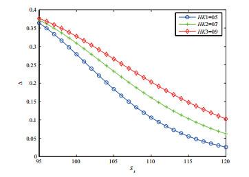
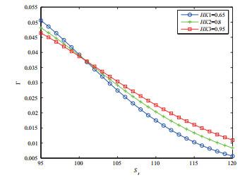
Among many risk characteristic parameters,

Δ = \frac{\partial C_{t}}{\partial S_{t}}

and

Γ = \frac{\partial^{2} C_{t}}{\partial S_{t}^{2}}

are the two most important indexes of option pricing sensitivity.

Δ

is the slope of the option value, also known as the hedging ratio, which accurately defines how many units the option price will change when the underlying asset price changes by one unit. This sensitivity is what option investors are most concerned about. When constructing the risk-free arbitrage asset portfolio, the ratio of the underlying asset held by the investor to the option position is

Δ

Γ

is the curve of the option value line. The larger

Γ

is, the harder it is to avoid risk. In this paper, the Black-Scholes option pricing model is taken as an example to analyze the risk characteristics. According to formula (10), the two hedging parameters can be deduced as follows:

\begin{array}{rcl} Δ = Φ (d_{1}), \end{array}

(30)

\begin{array}{rcl} Γ = \frac{1}{S_{t} σ \sqrt{T^{2 H K} - t^{2 H K}}} φ (d_{1}), \end{array}

(31)

where

φ (x) = \frac{1}{\sqrt{2 π}} e^{- \frac{x^{2}}{2}}

We take a first look at the value of

Δ

for different parameters

H K

. Apparently, in the case displayed in Figure 1, an increasing parameter comes along with a increasing of the value of

Δ

. Noticed that the value of

Δ

is positive, which is consistent with the characteristics of European call options. It's easy to see that the value of

Δ

is negative when the option is European put option.

Figure 1 The value of $Δ$ with varying parameter $H K$ ( $r = 0.03, k = 95, σ = 0.1, T = 2, t = 0.5$ )

Full size|PPT slide

Figure 2 indicates that

Γ

decreases with the increase of

H K

when the price of the underlying asset

S_{t}

is not much different from the exercise price

k

. When

S_{t}

differs greatly from

k

Γ

is proportional to

H K

. This indicates that the investors are more willing to exercise this option when the difference between

S_{t}

and

k

is large, otherwise, this option will not be exercised.

Figure 2 The value of $Γ$ with varying parameter $H K$ ( $r = 0.03, k = 95, σ = 0.1, T = 2, t = 0.5$ )

Full size|PPT slide

6 Conclusions

A large number of scholars have shown that the price volatility of financial assets has a long memory, which leads to the improvement of option pricing model based on Brownian motion hypothesis. In this paper, the Black-Scholes option pricing formula driven by bifractional Brownian motion is solved by Delta hedging strategy. Furthermore, we study the European options and the compound options driven by the bifractional Brownian motion respectively. By comparing the fluctuation of risk characteristics under different

H K

values, it is found that European call options with higher long memory parameter

H K

are more conducive to investors to implement effective hedging strategies.

References

Publishing order | Descend order by publishing year | Descend order by cited within

1	Black F, Scholes M. The pricing of options and corporate liabilities. Journal of Political Economy, 1973, 81 (3): 637- 657. https://doi.org/10.1086/260062 Cited in this article [1]

2	Peters E E. Fractal structure in the capital markets. Financial Analysts Journal, 1989, 7 (32): 434- 453. Cited in this article [1]

3	Lin S J. Stochastic analysis of fractional Brownian motions. Stochastics—An International Journal of Probability and Stochastic Processes, 1995, 55 (1/2): 121- 140. Cited in this article [1]

4	Bender C, Elliott R J. Arbitrage in a discrete version of the Wick-fractional Black-Scholes market. Mathematics of Operations Research, 2004, 29 (4): 935- 945. https://doi.org/10.1287/moor.1040.0096 Cited in this article [1]

5	Björk T, Hult H. A note on Wick products and the fractional Black-Scholes model. Finance and Stochastics, 2005, 9 (2): 197- 209. https://doi.org/10.1007/s00780-004-0144-5 Cited in this article [1]

6	Xiao W L, Zhang W G, Zhang X L, et al. Pricing model for equity warrants in a mixed fractional Brownian environment and its algorithm. Physica A: Statistical Mechanics and Its Applications, 2012, 391 (24): 6418- 6431. https://doi.org/10.1016/j.physa.2012.07.041 Cited in this article [1]

7	Sun L. Pricing currency options in the mixed fractional Brownian environment. Physica A: Statistical Mechanics and Its Applications, 2013, 392 (16): 3441- 3458. https://doi.org/10.1016/j.physa.2013.03.055

8	Shokrollahi F, Kılıçman A. Actuarial approach in a mixed fractional Brownian motion with jumps environment for pricing currency option. Advances in Difference Equations, 2015, 2015 (1): 257. https://doi.org/10.1186/s13662-015-0590-8 Cited in this article [1]

9	Lei P, Nualart D. A decomposition of the bifractional Brownian motion and some applications. Statistics and Probability Letters, 2008, 79 (5): 619- 624. Cited in this article [1]

10	Russo F, Tudor C. On the bifractional Brownian motion. Stochastic Processes and their Applications, 2006, 116 (5): 830- 856. https://doi.org/10.1016/j.spa.2005.11.013 Cited in this article [1]

11	Es-Sebaiy K, Tudor C. Multidimentsional bifractional Brownian motion: Itô and Tanaka's formulas. Stochastics and Dynamics, 2007, 7 (3): 365- 388. https://doi.org/10.1142/S0219493707002050 Cited in this article [1]

12	Xiao W L, Zhang W G, Xu W D. Pricing equity warrants in a bifractional Brownian motion. Journal of Systems Engineering, 2013, 28 (3): 348- 354. Cited in this article [1]

13	Zhao W. Research on depressed option pricing driven by bifractional Brownian motion. Journal of Nanjing University (Natural Science Edition), 2017, 40 (4): 21- 25. Cited in this article [1]

14	Song R L, Li X, Wang W. Asian option pricing in double fractional Brownian model with Markovian switching. Journal of Chongqing Technology and Business University (Natural Science Edition), 2019, 36 (1): 73- 77. Cited in this article [1]

15	Chen Z L, Sang L H, Hao X Z. Renormalized self-intersection local time of bifractional Brownian motion. Journal of Inequalities and Applications, 2018, 2018 (1): 1- 20. https://doi.org/10.1186/s13660-017-1594-6 Cited in this article [1]

16	Ait Ouahra M, Ouahhabi H, Sghir A. Continuity in law of some additive functionals of bifractional Brownian motion. Stochastics, 2019, 91 (4): 613- 628. https://doi.org/10.1080/17442508.2019.1568436

17	Qin X, Lin X, Shang Q. Fuzzy pricing of binary option based on the long memory property of financial markets. Journal of Intelligent and Fuzzy Systems, 2020, 2020 (3): 1- 12. Cited in this article [1]

18	Geske R. The valuation of compound options. Journal of Financial Economics, 1979, 7 (1): 63- 81. https://doi.org/10.1016/0304-405X(79)90022-9 Cited in this article [1]

19	Gukhal C R. The compound option approach to American options on jump-diffusions. Journal of Economic Dynamics and Control, 2004, 28 (10): 2055- 2074. https://doi.org/10.1016/j.jedc.2003.06.002 Cited in this article [1]

20	Gong P, He Z W, Zhu S P. Pricing convertible bonds based on a multi-stage compound option model. Physica A: Statistical Mechanics and Its Applications, 2006, 366 (1): 449- 462. Cited in this article [1]

21	Ivanov R V, Ano K. Option pricing in time-changed Lévy models with compound Possion jumps. Modern Stochastics: Theory and Applications, 2019, 6 (1): 81- 107. Cited in this article [1]

22	Bender C, Sottine T, Valkeila E. Arbitrage with fractional Brownian motion. Theory of Stochastic Processes, 2006, 12 (3): 1- 12. Cited in this article [1]

Funding

the Fundamental Research Funds for Suzhou Vocational University of China(SVU2018YY01)

"QINGLAN" project of SVU

PDF(167 KB)

197

Accesses

Citation

Detail

Sections

Recommended

Abstract
Key words
Cite this article
1 Introduction
2 Preliminaries
3 The Bifractional Black-Scholes Equation for European Options
4 The Pricing Formulas of Compound Options
5 Numerical Simulation Analysis of Risk Characteristics
Figure 1 The value of $Δ$ with varying parameter $H K$ ( $r = 0.03, k = 95, σ = 0.1, T = 2, t = 0.5$ )
Figure 2 The value of $Γ$ with varying parameter $H K$ ( $r = 0.03, k = 95, σ = 0.1, T = 2, t = 0.5$ )
6 Conclusions
References
Funding

Received	Accepted	Published
2019-11-16	2020-06-01	2020-08-25
Issue Date
2020-08-25

Please choose a citation manager

Content to export

Abstract

Key words

Cite this article

1 Introduction

2 Preliminaries

3 The Bifractional Black-Scholes Equation for European Options

4 The Pricing Formulas of Compound Options

5 Numerical Simulation Analysis of Risk Characteristics

Figure 1 The value of $Δ$ with varying parameter $H K$ ( $r = 0.03, k = 95, σ = 0.1, T = 2, t = 0.5$ )

Figure 2 The value of $Γ$ with varying parameter $H K$ ( $r = 0.03, k = 95, σ = 0.1, T = 2, t = 0.5$ )

6 Conclusions

{{custom_sec.title}}

{{custom_sec.title}}

References

{{custom_fnGroup.title_en}}

Footnotes

Funding

Share

模态框（Modal）标题

Please choose a citation manager

Content to export

Abstract

Key words

Cite this article

1 Introduction

2 Preliminaries

3 The Bifractional Black-Scholes Equation for European Options

4 The Pricing Formulas of Compound Options

5 Numerical Simulation Analysis of Risk Characteristics

Figure 1 The value of Δ with varying parameter HK (r=0.03,k=95,σ=0.1,T=2,t=0.5)

Figure 2 The value of Γ with varying parameter HK (r=0.03,k=95,σ=0.1,T=2,t=0.5)

6 Conclusions

{{custom_sec.title}}

{{custom_sec.title}}

References

{{custom_fnGroup.title_en}}

Footnotes

Funding

Figure 1 The value of $Δ$ with varying parameter $H K$ ( $r = 0.03, k = 95, σ = 0.1, T = 2, t = 0.5$ )

Figure 2 The value of $Γ$ with varying parameter $H K$ ( $r = 0.03, k = 95, σ = 0.1, T = 2, t = 0.5$ )