Recursive Solution of Queue Length Distribution for Geo/G/1 Queue with Delayed Min(N, D)-Policy

Yingyuan WEI; Yinghui TANG; Miaomiao YU

doi:10.21078/JSSI-2020-367-20

PDF(331 KB)

Journal of Systems Science and Information ›› 2020, Vol. 8 ›› Issue (4) : 367-386. DOI: 10.21078/JSSI-2020-367-20

Recursive Solution of Queue Length Distribution for Geo/G/1 Queue with Delayed Min(N, D)-Policy

Author information +

History +

Abstract

In this paper we consider a discrete-time Geo/G/1 queue with delayed Min(N, D)-policy. Using renewal process theory, total probability decomposition technique and z-transform, we study the transient and equilibrium properties of the queue length from an arbitrary initial state, and obtain both the recursive expressions of the transient state queue length distribution and the steady state queue length distribution at arbitrary time epoch n⁺. Furthermore, we derive the important relations between equilibrium queue length distributions at different time epochs n^-, n and n⁺. Finally, we give some numerical examples about capacity decision in queueing systems to demonstrate the application of the analytical results reported in this paper.

Key words

delayed Min(N, D)-policy discrete-time queue / total probability decomposition technique / z-transform / queue length distribution / system capacity optimum design

Cite this article

EndNote

Ris (Procite)

Bibtex

Download Citations

Yingyuan WEI , Yinghui TANG , Miaomiao YU. Recursive Solution of Queue Length Distribution for Geo/G/1 Queue with Delayed Min(N, D)-Policy. Journal of Systems Science and Information, 2020, 8(4): 367-386 https://doi.org/10.21078/JSSI-2020-367-20

1 Introduction

Parallel to continuous-time queues, discrete-time queues are more suitable to model and analyze the digital communication system, and thus it has gained importance due to its applicability in the performance analysis of telecommunication systems. Classical examples are synchronous communication systems (slotted ALOHA) or packet switching systems with time slotting. Currently, ATM multiplexer in the broadband integrated services digital network (B-ISDN), circuit-switched time-division multiple access (TDMA) systems and slotted carrier-sense multiple access (CSMA) protocols have become a powerful incentive for the study of discrete-time queueing systems.

Queueing systems with control policies have been well studied by numerous researcher. Earliest works were the

N

-policy of Yadin and Naor^[1], the

D

-policy of Balachandran^[2] and the

T

-policy of Heyman^[3]. Since their seminal works, an enormous number of works on the threshold policies and vacation queues have been published.

As is well known, the

N

-policy stipulates that the idle server begins to serve the customers only when

N

customers have accumulated in the system. Under the

D

-policy, the idle server begins to operate when the total workload (i.e., the sum of the service times of the waiting customers) exceeds

D

. Under the

T

-policy, the server takes a vacation of fixed length

T

. After the server returns from vacation, he begins to serve the customers if there is one or more present. If not, he takes another vacation of length

T

. The process repeats in this way until the server finds at least one customer upon the return from a vacation. If

T

is a random variable, the system becomes the multiple vacation system of Levy and Yechiali^[4].

N

-policy is most often combined with vacations. Hur and Paik^[5] studied the effect of different arrival rates on the

N

-policy M/G/1 queue with server setup, and derived the steady state queue length, waiting time and the optimal value of

N

. Wang and Huang^[6] analyzed the

⟨ p, N ⟩

-policy M/G/1 queue with a removable and unreliable server, and used the maximum entropy approach to develop the approximate formulae for the probability distributions of the number of customers and the expected waiting time in the system. Tang, et al.^[7] studied the queue size of M/G/1 queueing system with

N

-policy and setup times. As for discrete time case, Wei, et al.^[8] considered the Geo/G/1 queueing system with delayed

N

-policy. Recently, Wei, et al.^[9] further investigated the

N

-policy queue with setup time and variable input rate. The recursive expressions of the

z

-transformation of the transient queue length distribution and the recursive expressions of the steady state queue length distribution at arbitrary time epoch are both obtained. Luo, et al.^[10] obtained the recursive solution of queue length for Geo/G/1 queue with

N

-policy, and the important relations between the steady state queue length distributions at different time epochs

n^{-}

n

and

n^{+}

are discovered. Moreover, under the renewal input process, Lim, et al.^[11] studied the GI/Geo/1 queue with

N

-policy, the steady state queue length and the waiting time distributions are derived by them.

The pioneering works on the analysis of M/G/1 queue with

D

-policy were carried out by Chae and Park^[12] and Artalejo^[13]. More works concerning

D

-policy can be found in Lee and Beak^[14], Wang^[15], Lee, et al.^[16], and Wei, et al.^[17].

Recently, most works on the dynamic control of the queueing systems are concerned with joint policies where two or more policies are combined. Lee and Seo^[18] considered the M/G/1 queue under the Min

(N, D)

-policy and performed some cost optimization. Lee, et al.^[19] considered the MAP/G/1 queue under the Min

(N, D)

-policy and analyzed the queue length, workload, and waiting time. Tang, et al.^[20] studied the M/G/1 queueing system with Min

(N, V)

-policy based on multiple server vacations and obtained the queue length distribution.

In this paper, we consider the discrete-time Geo/G/1 queue under the delayed Min

(N, D)

-policy. To the best of the authors' knowledge, this paper is the first study on the discrete-time Geo/G/1 queue under the delayed Min

(N, D)

-policy.

The consideration of delayed Min

(N, D)

-policy is not only for generalization in mathematics. In fact, it approximates some real world situations more closely. For example, this sort of queue occurs in the area of transportation systems. In a courier service a worker usually needs some preparation and duty-transition procedure besides his/her primary express delivery service. The preparation and duty-transition procedure are needed to improve efficiency. It is desirable that a truck serving a particular origin-destination pair should carry more than one package on a trip. Hence, if there is less than

N

packages waiting it waits until the

N

-th package arrives. However, in order to maintain good business it does not want to keep packages delayed too long if there is not up to

N

available. Hence, if the total backlog of the delivery service time of the waiting packages exceeds

D

the truck departs even if there is less than

N

packages.

In this paper, we firstly define server busy period and system idle period respectively, and discuss the probability distribution of the transient state queue length in a server busy period by employing the total probability decomposition technique. Then starting from an arbitrary initial state, we discuss the probability distribution of the transient state queue length at arbitrary time epoch

n^{+}

and also report the recursive expression for the steady state queue length distribution. It is worthwhile to point out that through the traditional analysis techniques (e.g., embedded Markov chain and supplementary variable techniques) it is very difficult to obtain the recursive expression of the steady state queue length distribution. More importantly, in contrast to the traditional methods, using the analysis technique proposed in this paper, we can easily obtain the recursive formulas of the steady state queue length distribution that are more suited for numerical computations. Furthermore, with the

z

-transform technique, we derive the probability generating functions of the transient and the steady state distributions of the queue length. Especially, we can obtain some corresponding results of the discrete-time queueing system under some special cases. Finally, by numerical examples, we investigate the sensitivity of variant system parameters on the stationary queue length distribution, and also illustrate the applications of the stationary queue length distribution in the system capacity design.

The rest of the paper is organized as follows. In the next section, the model of the considered queueing system is described. In Section 3, we study the transient state queue length distribution at time epoch

n^{+}

during the server busy period. In Section 4, we study the transient state distribution and the steady state distribution of the queue size at arbitrary time epoch

n^{+}

. Moreover, we also find that the queue length distribution in equilibrium follows the stochastic decomposition discipline under the Min

(N, D)

-policy. In Section 5, we study the steady state queue length distribution at time epochs

n^{-}

and

n

, and give the important relationship between the steady state queue length distributions at different epochs

n^{-}

n

and

n^{+}

. In Section 6, we demonstrate that several queue models are special cases of the queueing model presented in this study. Finally, we give numerical examples in Section 7.

2 Model Formulation

We consider a discrete-time Geo/G/1 queueing system with delayed Min

(N, D)

-policy. The arrivals at different times are independent from each other. The customers are served one by one. For mathematical clarity, we assume that the model discussed in this paper is a late arrival system with delayed access (LAS-DA) ^[21], that is, a potential arrival can only take place in

(n^{-}, n)

n = 0, 1, \dots

, a potential service and departure can only take place in

(n, n^{+})

n = 1, 2, \dots

. We do not permit a departure at such a time point for a customer who has just arrived the instant previously to an empty system. Furthermore, we suppose that there is no customer arrival in the beginning time interval

(0^{-}, 0)

and no departure in

(0, 0^{+})

The time between two successive arrivals, denoted by

τ

follows a geometric distribution with parameter

p

, and probability mass function (p.m.f.)

P {τ = j} = p (1 - p)^{j - 1}

j = 1, 2, \dots

0 < p < 1

. That is to say, a customer arrives with probability

p

in each interval

(n^{-}, n)

n = 0, 1, \dots

, and the probability that no customer arrives is

1 - p

. The service times, denoted by

χ_{i} (i = 1, 2, \dots)

, are independent and identically distributed (i.i.d.) random variables with p.m.f.

P {χ = j} = g_{j}

j = 1, 2, \dots

, and the probability generating function (p.g.f.)

G (z) = \sum_{j = 1}^{\infty} g_{j} z^{j}, | z | < 1

. The average service time is finite and denoted by

μ (1 ⩽ μ < \infty)

The policy of this queueing system is delayed Min

(N, D)

-policy. Whenever the system becomes empty, the server (being in his/her post) will spend some time for preparation and duty-transition procedure before he/she begins to server the customs. The preparation and duty-transition procedure are needed to provide high reliability and improve the system performance. If customers arrive in the preparation (delayed) time, the server will begin to serve the customs immediately until there are no customers remaining in the queue. The length of the delayed time, denoted by

Y

, is generally distributed. The delayed times are independent and identically distributed (i.i.d.) random variables with p.m.f.

P {Y = j} = y_{j}

j = 0, 1, \dots

, and p.g.f.

Y (z) = \sum_{j = 0}^{\infty} y_{j} z^{j}

| z | < 1

, and finite mean

E (Y) (0 ⩽ E (Y) < \infty)

and variance. If no customer arrives in delayed time, the idle server resumes its service if either one of the following two conditions is met, whichever occurs first:

(i)

N

customers have accumulated in the system, or

(ii) total backlog of the service time of the waiting customers exceeds

D

where

N

and

D

denote fixed positive integer, i.e.,

N, D \in Z^{+}, Z^{+}

denotes the set of positive integer.

Various stochastic processes involved in the system are assumed to be independent of each other. Furthermore, we suppose that the service begins at once if there are

k (k ⩾ 1)

customers at initial epoch

0^{+}

(this assumption has no effect on the steady state queue length distribution).

In this paper, let

L (n^{-})

L (n)

and

L (n^{+})

denote the queue length at time epochs

n^{-}

n

and

n^{+}

, e.g., the number of customers present in the system (including the one in service) at time epochs

n^{-}, n

and

n^{+}

, respectively.

R

denotes the set of real number.

\bar{p} = 1 - p, f (z) = \frac{p z}{1 - \bar{p} z}, min {a, b} = {\begin{array}{cc} a, & a \leq b, \\ b, & a > b, \end{array} a, b \in R .

3 Recursive Solution for Transient State Queue Length Distribution at Time Epoch $n^{+}$ During Server Busy Period

For mathematical clarity, we note that "server busy period" is from the instant when the server begins to serve customers until the system becomes idle again. Let

b

represent the length of server busy period initiated by only one customer. We have the following Lemma which is also give by Bruneel and Kim^[22].

Lemma 1 Let $B (z) = \sum_{j = 1}^{\infty} P {b = j} z^{j}, | z | < 1$ , then $B (z)$ subjects to the equation $B (z) = G ((1 - p + p B (z)) z)$ , mean

E [b] = {\begin{cases} \frac{ρ}{p (1 - ρ)}, & ρ < 1, \\ \infty, & ρ ⩾ 1, \end{cases}

where $ρ = p μ$ .

Let

b^{⟨ i ⟩}

denote the server busy period initiated by

i

customers, because of the Markovian property of geometric distribution,

b^{⟨ i ⟩}

can be expressed as

b^{⟨ i ⟩} = b_{1} + b_{2} + \dots + b_{i}, i = 1, 2, \dots,

where

b_{1}, b_{2}, \dots, b_{i}

are independent of each other, and have the same distribution function as

b

, therefore

\sum_{j = i}^{\infty} P {b^{⟨ i ⟩} = j} z^{j} = B^{i} (z), i = 1, 2, \dots, | z | < 1.

"System idle time" is from the instant when the system becomes idle until a new customer arrives. The system idle time of the queueing system is the residual time of arriving interval.

In the remaining part of this section, we will give the distribution of the queue length at time epoch

n^{+}

during the server busy period

b

. Let

Q_{j} (n^{+}) = P {b > n^{+}, L (n^{+}) = j}, j = 1, 2, \dots

represent the probability that the queueing length equals to

j

at instant

n^{+}

during server busy period

b

, where the instant

n^{+} = 0^{+}

is the beginning of the busy period

b

, and the boundary condition is

Q_{1} (0^{+}) = 1, Q_{j} (0^{+}) = 0, j = 2, 3, \dots

Lemma 2 If $| z | < 1$ , let $q_{j}^{+} (z) = \sum_{n = 0}^{\infty} Q_{j} (n^{+}) z^{n}$ present the p.g.f. of $Q_{j} (n^{+})$ , hence we have the following recursive expressions of $q_{j}^{+} (z)$ ,

\begin{aligned} q_{1}^{+} (z) = & \frac{B (z) [1 - G (\bar{p} z)]}{[1 - \bar{p} z] G (\bar{p} z)}, \\ q_{j}^{+} (z) = & \frac{1}{G (\bar{p} z)} {B (z) \sum_{n = j - 1}^{\infty} z^{n} \sum_{k = n + 1}^{\infty} g_{k} (\binom{n}{j - 1}) p^{j - 1} {\bar{p}}^{n - j + 1} \\ + \sum_{i = 1}^{j - 1} \frac{q_{j - i}^{+} (z)}{B^{i} (z)} [B (z) - G (\bar{p} z) - \sum_{m = 1}^{i} \sum_{k = m}^{\infty} (\binom{k}{m}) g_{k} z^{k} (p B (z))^{m} {\bar{p}}^{k - m}]}, j = 2, 3, \dots, \end{aligned}

where $\sum_{i = 1}^{j} = 0$ if $j ⩽ 0$ .

Proof The proof is similar to Theorem 2.1 in [23].

4 Solution for Transient State and Steady State Queue Length Distribution at Time Epoch $n^{+}$

One of the important operating characteristics in a queueing system is the queue length distribution. In the following subsections, using a new method, we will study the system queue length at different time epochs.

Let

P_{i j} (n^{+}) = P {L (n^{+}) = j | L (0^{+}) = i} (i, j = 0, 1, \dots)

be the conditional probability of the queue length, and

p_{i j}^{+} (z) = \sum_{n = 0}^{\infty} P_{i j} (n^{+}) z^{n}

represents the p.g.f. of

P_{i j} (n^{+})

. Since the system is renewal process alternates with server busy period and server idle period, by using renewal process theory and total probability decomposition technique, we obtain the recursive expression of the

z

-transformation of the transient queue length distribution at any time epoch

n^{+}

as follows.

Theorem 1 When $N = 1$ and $P {Y = 0} = 1$ , or $D = 1$ and $P {Y = 0} = 1$ , if $| z | < 1$ , then we have

\begin{aligned} p_{i 0}^{+} (z) & = \frac{[B (z)]^{i}}{1 - \bar{p} z - p z B (z)}, i = 0, 1, \dots, \end{aligned}

(1)

\begin{aligned} p_{0 j}^{+} (z) & = \frac{p z q_{j}^{+} (z)}{1 - \bar{p} z - p z B (z)}, j = 1, 2, \dots, \end{aligned}

(2)

\begin{aligned} p_{i j}^{+} (z) & = \sum_{k = 1}^{i} B^{k - 1} (z) q_{j - i + k}^{+} (z) + \frac{p z [B (z)]^{i} q_{j}^{+} (z)}{1 - \bar{p} z - p z B (z)}, i, j = 1, 2, \dots, \end{aligned}

(3)

where $B (z)$ and $q_{j}^{+} (z)$ are determined by Lemmas $1$ and $2$ , respectively.

Proof When

N = 1

and

P {Y = 0} = 1

D = 1

and

P {Y = 0} = 1

, the model discussed in this paper becomes the classical Geo/G/1 queueing system. Thus the process of deduction is similar to the proof in [23].

Theorem 2 When $N \geq 2$ and $D \geq 2, N, D \in Z^{+}$ , if $| z | < 1$ , then $p_{00}^{+} (z)$ and $p_{i 0}^{+} (z)$ are given by

\begin{aligned} p_{00}^{+} (z) & = \frac{1}{1 - \bar{p} z} {1 + \frac{f (z) B (z)}{Δ (z)}}, \end{aligned}

(4)

\begin{aligned} p_{i 0}^{+} (z) & = \frac{[B (z)]^{i}}{[1 - \bar{p} z] Δ (z)}, i = 1, 2, \dots, \end{aligned}

(5)

where $B (z)$ is determined by Lemma $1$ ,

\begin{array}{rcl} min {N - 1, D} = {\begin{array}{cc} N - 1, & N - 1 \leq D, \\ D, & N - 1 > D, \end{array} \\ C_{m} (D) = P {\sum_{s = 1}^{m} χ_{s} < D}, C_{0} (D) = 1, \\ A_{m} (D) = C_{m - 1} (D) - C_{m} (D), m = 1, 2, \dots, min {N - 1, D}, \\ Δ (z) = 1 - f (z) B (z) + Y (\bar{p} z) {f (z) B (z) - C_{N - 1} (D) [f (z) B (z)]^{N} \\ - \sum_{m = 1}^{min {N - 1, D}} A_{m} (D) [f (z) B (z)]^{m}} . \end{array}

Proof Let

S_{k} = \sum_{i = 1}^{k} χ_{i}, l_{k} = \sum_{i = 1}^{k} τ_{i}

, and

S_{0} = l_{0} = 0

. The system is empty at time epoch

n^{+}

if and only if the system is in the "system idle period". Because all of the beginning and ending epochs of server busy period are renewal points, by using renewal process theory and total probability decomposition technique, the conditional probability

P_{00} (n^{+})

can be divided into two parts according to whether the first customer arrived before

n^{+}

. Given that system starts from idle state, we have

\begin{aligned} P_{00} (n^{+}) = & P {0 \leq n^{+} < {\hat{τ}}_{1}} + P {{\hat{τ}}_{1} + b \leq n^{+} < {\hat{τ}}_{1} + b + {\hat{τ}}_{2}} \\ + P {0 < {\hat{τ}}_{2} \leq Y, {\hat{τ}}_{1} + b + {\hat{τ}}_{2} \leq n^{+}, L (n^{+}) = 0} \\ + \sum_{m = 1}^{min {N - 1, D}} P {{\hat{τ}}_{2} > Y \geq 0, {\hat{τ}}_{1} + b + {\hat{τ}}_{2} + l_{m - 1} \leq n^{+}, S_{m - 1} < D \leq S_{m}, L (n^{+}) = 0} \\ + P {{\hat{τ}}_{2} > Y \geq 0, {\hat{τ}}_{1} + b + {\hat{τ}}_{2} + l_{N - 1} \leq n^{+}, S_{N - 1} < D, L (n^{+}) = 0} \\ = & {\bar{p}}^{n} + \sum_{t = 2}^{n} P {{\hat{τ}}_{1} + b = t} {\bar{p}}^{n - t} \\ + \sum_{t = 2}^{n - 1} P {{\hat{τ}}_{1} + b = t} \sum_{r = 1}^{n - t} P {{\hat{τ}}_{2} = r} \sum_{l = r}^{\infty} P {Y = l} P_{10} ((n - t - r)^{+}) \\ + \sum_{m = 1}^{min {N - 1, D}} A_{m} (D) \sum_{t = 2}^{n - m} P {{\hat{τ}}_{1} + b = t} \sum_{r = 1}^{n - t - m + 1} P {{\hat{τ}}_{2} = r} \sum_{l = 0}^{r - 1} P {Y = l} \\ \cdot \sum_{u = m - 1}^{n - t - r} P {l_{m - 1} = u} P_{m 0} ((n - t - r - u)^{+}) \\ + C_{N - 1} (D) \sum_{t = 2}^{n - N} P {{\hat{τ}}_{1} + b = t} \sum_{r = 1}^{n - t - N + 1} P {{\hat{τ}}_{2} = r} \sum_{l = 0}^{r - 1} P {Y = l} \\ \cdot \sum_{u = N - 1}^{n - t - r} P {l_{N - 1} = u} P_{N 0} ((n - t - r - u)^{+}), \end{aligned}

(6)

where

{\hat{τ}}_{k}

denotes the

k

(k \geq 1)

"system idle time" that the system starts from the initial state

L (0^{+}) = 0, {\hat{τ}}_{k}

follows the same distribution as

τ

For

i = 1, 2, \dots

, similarly, we have

\begin{aligned} P_{i 0} (n^{+}) = & \sum_{t = i}^{n} P {b^{⟨ i ⟩} = t} {\bar{p}}^{n - t} \\ + \sum_{t = i}^{n - 1} P {b^{⟨ i ⟩} = t} \sum_{r = 1}^{n - t} P {{\hat{τ}}_{1} = r} \sum_{l = r}^{\infty} P {Y = l} P_{10} ((n - t - r)^{+}) \\ + \sum_{m = 1}^{min {N - 1, D}} A_{m} (D) \sum_{t = i}^{n - m} P {b^{⟨ i ⟩} = t} \sum_{r = 1}^{n - t - m + 1} P {{\hat{τ}}_{1} = r} \sum_{l = 0}^{r - 1} P {Y = l} \\ \cdot \sum_{u = m - 1}^{n - t - r} P {l_{m - 1} = u} P_{m 0} ((n - t - r - u)^{+}) \\ + C_{N - 1} (D) \sum_{t = i}^{n - N} P {b^{⟨ i ⟩} = t} \sum_{r = 1}^{n - t - N + 1} P {{\hat{τ}}_{1} = r} \sum_{l = 0}^{r - 1} P {Y = l} \\ \cdot \sum_{u = N - 1}^{n - t - r} P {l_{N - 1} = u} P_{N 0} ((n - t - r - u)^{+}) . \end{aligned}

(7)

Taking the p.g.f. on both sides of the equations

(6)

and

(7)

, respectively, we have

\begin{aligned} p_{00}^{+} (z) = & \frac{1}{1 - \bar{p} z} + f (z) B (z) {\frac{1}{1 - \bar{p} z} + f (z) [1 - Y (\bar{p} z)] p_{10}^{+} (z) \\ + Y (\bar{p} z) [C_{N - 1} (D) [f (z)]^{N} p_{N 0}^{+} (z) + \sum_{m = 1}^{min {N - 1, D}} A_{m} (D) [f (z)]^{m} p_{m 0}^{+} (z)]}, \end{aligned}

(8)

\begin{aligned} p_{i 0}^{+} (z) = & [B (z)]^{i} {\frac{1}{1 - \bar{p} z} + f (z) [1 - Y (\bar{p} z)] p_{10}^{+} (z) \\ + Y (\bar{p} z) [C_{N - 1} (D) [f (z)]^{N} p_{N 0}^{+} (z) + \sum_{m = 1}^{min {N - 1, D}} A_{m} (D) [f (z)]^{m} p_{m 0}^{+} (z)]} . \end{aligned}

(9)

Equations (8) and (9) give the relationship between

p_{00}^{+} (z)

and

p_{i 0}^{+} (z)

\begin{aligned} p_{i 0}^{+} (z) = \frac{[B (z)]^{i - 1}}{f (z)} [p_{00}^{+} (z) - \frac{1}{1 - \bar{p} z}], i = 1, 2, \dots . \end{aligned}

(10)

Substituting (10) into (8) gives (4), and furthermore, we get (5).

Theorem 3 When $N \geq 2$ and $D \geq 2, N, D \in Z^{+}$ , if $| z | < 1, i = 1, 2, \dots, j = 1, 2, \dots,$ $min {N, D} - 1$ , then $p_{0 j}^{+} (z)$ and $p_{i j}^{+} (z)$ are given by

\begin{aligned} p_{0 j}^{+} (z) = & f (z) {q_{j}^{+} (z) + \frac{γ_{j} (z)}{Δ (z)}}, \end{aligned}

(11)

\begin{aligned} p_{i j}^{+} (z) = & \sum_{k = 1}^{i} [B (z)]^{k - 1} q_{j - i + k}^{+} (z) + \frac{[B (z)]^{i - 1} γ_{j} (z)}{Δ (z)}, \end{aligned}

(12)

where $B (z)$ and $q_{j}^{+} (z)$ are determined by Lemmas $1$ and $2$ , respectively, $Δ (z)$ has been given in Theorem $2$ ,

\begin{aligned} γ_{j} (z) = & f (z) B (z) [1 - Y (\bar{p} z)] q_{j}^{+} (z) + Y (\bar{p} z) {\frac{C_{j} (D) [f (z)]^{j} B (z)}{1 - \bar{p} z} \\ + C_{N - 1} (D) [f (z)]^{N} \sum_{k = N - j + 1}^{N} [B (z)]^{k} q_{j - N + k}^{+} (z) + \sum_{m = 1}^{j} A_{m} (D) [f (z)]^{m} \sum_{k = 1}^{m} [B (z)]^{k} q_{j - m + k}^{+} (z) \\ + \sum_{m = j + 1}^{min {N - 1, D}} A_{m} (D) [f (z)]^{m} \sum_{k = m - j + 1}^{m} [B (z)]^{k} q_{j - m + k}^{+} (z)} . \end{aligned}

Proof For

j = 1, 2, \dots, min {N, D} - 1, L (n^{+}) = j

indicates that epoch

n^{+}

locates in server busy period or server idle period with some customers waiting for service, by using the same method as in the proof of Theorem 2, we have

\begin{aligned} P_{0 j} (n^{+}) = & P {{\hat{τ}}_{1} ⩽ n^{+} < {\hat{τ}}_{1} + b; L (n^{+}) = j} + P {0 < {\hat{τ}}_{2} \leq Y, {\hat{τ}}_{1} + b + {\hat{τ}}_{2} \leq n^{+}, L (n^{+}) = j} \\ + \sum_{m = 1}^{min {N - 1, D}} P {{\hat{τ}}_{2} > Y \geq 0, {\hat{τ}}_{1} + b + {\hat{τ}}_{2} + l_{j - 1} ⩽ n^{+} < {\hat{τ}}_{1} + b + {\hat{τ}}_{2} + l_{j}, \\ S_{j} < D, S_{m - 1} < D \leq S_{m}} \\ + \sum_{m = 1}^{min {N - 1, D}} P {{\hat{τ}}_{2} > Y \geq 0, {\hat{τ}}_{1} + b + {\hat{τ}}_{2} + l_{m - 1} ⩽ n^{+}, S_{m - 1} < D \leq S_{m}, L (n^{+}) = j} \\ + P {{\hat{τ}}_{2} > Y \geq 0, {\hat{τ}}_{1} + b + {\hat{τ}}_{2} + l_{j - 1} ⩽ n^{+} < {\hat{τ}}_{1} + b + {\hat{τ}}_{2} + l_{j}, S_{j} < D, S_{N - 1} < D} \\ + P {{\hat{τ}}_{2} > Y \geq 0, {\hat{τ}}_{1} + b + {\hat{τ}}_{2} + l_{N - 1} ⩽ n^{+}, S_{N - 1} < D, L (n^{+}) = j} \\ = & \sum_{t = 1}^{n} P {{\hat{τ}}_{1} = t} Q_{j} ((n - t)^{+}) \\ + \sum_{t = 2}^{n - 1} P {{\hat{τ}}_{1} + b = t} \sum_{r = 1}^{n - t} P {{\hat{τ}}_{2} = r} \sum_{l = r}^{\infty} P {Y = l} P_{1 j} ((n - t - r)^{+}) \\ + C_{j} (D) \sum_{t = 2}^{n - j} P {{\hat{τ}}_{1} + b = t} \sum_{r = 1}^{n - t - j + 1} P {{\hat{τ}}_{2} = r} \sum_{l = 0}^{r - 1} P {Y = l} \sum_{u = j - 1}^{n - t - r} P {l_{j - 1} = u} {\bar{p}}^{n - t - r - u} \\ + \sum_{m = 1}^{min {N - 1, D}} A_{m} (D) \sum_{t = 2}^{n - m} P {{\hat{τ}}_{1} + b = t} \sum_{r = 1}^{n - t - m + 1} P {{\hat{τ}}_{2} = r} \sum_{l = 0}^{r - 1} P {Y = l} \\ \cdot \sum_{u = m - 1}^{n - t - r} P {l_{m - 1} = u} P_{m j} ((n - t - r - u)^{+}) \\ + C_{N - 1} (D) \sum_{t = 2}^{n - N} P {{\hat{τ}}_{1} + b = t} \sum_{r = 1}^{n - t - N + 1} P {{\hat{τ}}_{2} = r} \sum_{l = 0}^{r - 1} P {Y = l} \\ \cdot \sum_{u = N - 1}^{n - t - r} P {l_{N - 1} = u} P_{N j} ((n - t - r - u)^{+}), \end{aligned}

(13)

where

{\hat{τ}}_{k}, k \geq 1

has been given in Theorem 2.

For

L (0^{+}) = i, i = 1, 2, \dots

, similarly, we have

\begin{aligned} P_{i j} (n^{+}) = & \sum_{k = 1}^{i} \sum_{r = k - 1}^{n} P {b_{1} + b_{2} + \dots + b_{k - 1} = r} Q_{j - i + k} ((n - r)^{+}) \\ + \sum_{t = i}^{n - 1} P {b^{⟨ i ⟩} = t} \sum_{r = 1}^{n - t} P {{\hat{τ}}_{1} = r} \sum_{l = r}^{\infty} P {Y = l} P_{1 j} ((n - t - r)^{+}) \\ + C_{j} (D) \sum_{t = i}^{n - j} P {b^{⟨ i ⟩} = t} \sum_{r = 1}^{n - t - j + 1} P {{\hat{τ}}_{1} = r} \sum_{l = 0}^{r - 1} P {Y = l} \\ \cdot \sum_{u = j - 1}^{n - t - r} P {l_{j - 1} = u} {\bar{p}}^{n - t - r - u} \\ + \sum_{m = 1}^{min {N - 1, D}} A_{m} (D) \sum_{t = i}^{n - m} P {b^{⟨ i ⟩} = t} \sum_{r = 1}^{n - t - m + 1} P {{\hat{τ}}_{1} = r} \sum_{l = 0}^{r - 1} P {Y = l} \\ \cdot \sum_{u = m - 1}^{n - t} P {l_{m - 1} = u} P_{m j} ((n - t - r - u)^{+}) \\ + C_{N - 1} (D) \sum_{t = i}^{n - N} P {b^{⟨ i ⟩} = t} \sum_{r = 1}^{n - t - N + 1} P {{\hat{τ}}_{1} = r} \sum_{l = 0}^{r - 1} P {Y = l} \\ \cdot \sum_{u = N - 1}^{n - t - r} P {l_{N - 1} = u} P_{N j} ((n - t - r - u)^{+}) . \end{aligned}

(14)

Taking the p.g.f. on both sides of Equations (13) and (14), respectively, we have

\begin{aligned} p_{0 j}^{+} (z) & = f (z) q_{j}^{+} (z) + f (z) B (z) {f (z) [1 - Y (\bar{p} z)] p_{1 j}^{+} (z) + Y (\bar{p} z) [C_{N - 1} (D) [f (z)]^{N} p_{N j}^{+} (z) \\ + \sum_{m = 1}^{min {N - 1, D}} A_{m} (D) [f (z)]^{m} p_{m j}^{+} (z) + \frac{C_{j} (D) [f (z)]^{j}}{1 - \bar{p} z}]}, \end{aligned}

(15)

\begin{aligned} p_{i j}^{+} (z) & = \sum_{k = 1}^{i} [B (z)]^{k - 1} q_{j - i + k}^{+} (z) \\ + [B (z)]^{i} {f (z) [1 - Y (\bar{p} z)] p_{1 j}^{+} (z) + Y (\bar{p} z) [C_{N - 1} (D) [f (z)]^{N} p_{N j}^{+} (z) \\ + \sum_{m = 1}^{min {N - 1, D}} A_{m} (D) [f (z)]^{m} p_{m j}^{+} (z) + \frac{C_{j} (D) [f (z)]^{j}}{1 - \bar{p} z}]} . \end{aligned}

(16)

With

(15)

and

(16)

, we can get the relationship between

p_{0 j}^{+} (z)

and

p_{i j}^{+} (z)

\begin{aligned} p_{i j}^{+} (z) = \sum_{k = 1}^{i} [B (z)]^{k - 1} q_{j - i + k}^{+} (z) + \frac{[B (z)]^{i - 1}}{f (z)} {p_{0 j}^{+} (z) - f (z) q_{j}^{+} (z)}, \\ i = 1, 2, \dots, j = 1, 2, \dots, min {N, D} - 1. \end{aligned}

(17)

Substituting

(17)

into

(15)

gives

(11)

, and furthermore, we get

(12)

Theorem 4 When $N \geq 2$ and $D \geq 2, N, D \in Z^{+}$ , if $| z | < 1, i = 1, 2, \dots, j = min {N, D},$ $min {N, D} + 1, min {N, D} + 2, \dots,$ then $p_{0 j}^{+} (z)$ and $p_{i j}^{+} (z)$ are given by

\begin{aligned} p_{0 j}^{+} (z) = & f (z) {q_{j}^{+} (z) + \frac{σ_{j} (z)}{Δ (z)}}, \end{aligned}

(18)

\begin{aligned} p_{i j}^{+} (z) = & \sum_{k = 1}^{i} [B (z)]^{k - 1} q_{j - i + k}^{+} (z) + \frac{[B (z)]^{i - 1} σ_{j} (z)}{Δ (z)}, \end{aligned}

(19)

where $B (z)$ and $q_{j}^{+} (z)$ are determined by Lemmas $1$ and $2$ , respectively, $Δ (z)$ has been given in Theorem $2$ ,

\begin{aligned} σ_{j} (z) = & f (z) B (z) [1 - Y (\bar{p} z)] q_{j}^{+} (z) + Y (\bar{p} z) {C_{N - 1} (D) [f (z)]^{N} \sum_{k = 1}^{N} [B (z)]^{k} q_{j - N + k}^{+} (z) \\ + \sum_{m = 1}^{min {N - 1, D}} A_{m} (D) [f (z)]^{m} \sum_{k = 1}^{m} [B (z)]^{k} q_{j - m + k}^{+} (z)} . \end{aligned}

Proof For

j = min {N, D}, min {N, D} + 1, min {N, D} + 2, \dots, L (n^{+}) = j

means that epoch

n^{+}

locates in server busy period with some customers waiting for service, the proof is similar to the Theorem 3.

Based on the transient state distribution of the queue length at arbitrary time epoch

n^{+}

obtained in Theorems 1 to 4, the steady state distribution of queue length at any time epoch

n^{+}

can be easily obtained as follows.

Theorem 5 Let $p_{j}^{+} = lim_{n \to \infty} P {L (n^{+}) = j}, j = 0, 1, \dots$ , when $N = 1$ and $P {Y = 0} = 1$ , or $D = 1$ and $P {Y = 0} = 1$ , we have

$1)$ when $ρ ⩾ 1$ , $p_{j}^{+} = 0, j = 0, 1, \dots$ .

$2)$ when $ρ < 1$ , ${p_{j}^{+}, j = 0, 1, \dots}$ exists and satisfies the following recursion formulas

\begin{aligned} p_{0}^{+} = & 1 - ρ, \end{aligned}

(20)

\begin{aligned} p_{1}^{+} = & \frac{(1 - ρ) (1 - G (\bar{p}))}{G (\bar{p})}, \end{aligned}

(21)

\begin{aligned} p_{j}^{+} = & \frac{1}{G (\bar{p})} {p (1 - ρ) \sum_{n = j - 1}^{\infty} \sum_{k = n + 1}^{\infty} g_{k} (\binom{n}{j - 1}) p^{j - 1} {\bar{p}}^{n - j + 1} \\ + \sum_{i = 1}^{j - 1} p_{j - i}^{+} [1 - G (\bar{p}) - \sum_{m = 1}^{i} \sum_{k = m}^{\infty} g_{k} p^{m} {\bar{p}}^{k - m}]}, i = 2, 3, \dots . \end{aligned}

(22)

Proof The proof is similar to Theorem 3.1 in [23].

Theorem 6 Let $p_{j}^{+} = lim_{n \to \infty} P {L (n^{+}) = j}, j = 0, 1, \dots$ , When $N \geq 2$ and $D \geq 2, N, D \in Z^{+},$ we have

$1)$ when $ρ ⩾ 1$ , $p_{j}^{+} = 0, j = 0, 1, \dots$ .

$2)$ when $ρ < 1$ , ${p_{j}^{+}, j = 0, 1, \dots}$ exists and satisfies the following recursion formulas

\begin{aligned} p_{0}^{+} = & \frac{1 - ρ}{1 + Y (\bar{p}) \sum_{m = 1}^{min {N, D} - 1} C_{m} (D)}, \end{aligned}

(23)

\begin{aligned} p_{j}^{+} = & p p_{0}^{+} {[1 - Y (\bar{p})] q_{j}^{+} (1) + Y (\bar{p}) [\frac{C_{j} (D)}{p} + C_{N - 1} (D) \sum_{k = N - j + 1}^{N} q_{j - N + k}^{+} (1) \\ + \sum_{m = 1}^{j} A_{m} (D) \sum_{k = 1}^{m} q_{j - m + k}^{+} (1) + \sum_{m = j + 1}^{min {N - 1, D}} A_{m} (D) \sum_{k = m - j + 1}^{m} q_{j - m + k}^{+} (1)]}, \\ j = 1, 2, \dots, min {N, D} - 1, \end{aligned}

(24)

\begin{aligned} p_{j}^{+} = & p p_{0}^{+} {[1 - Y (\bar{p})] q_{j}^{+} (1) + Y (\bar{p}) [C_{N - 1} (D) \sum_{k = 1}^{N} q_{j - N + k}^{+} (1) \\ + \sum_{m = 1}^{min {N - 1, D}} A_{m} (D) \sum_{k = 1}^{m} q_{j - m + k}^{+} (1)]}, \\ j = min {N, D}, min {N, D} + 1, min {N, D} + 2, \dots, \end{aligned}

(25)

where

\begin{aligned} q_{1}^{+} (1) = \frac{1 - G (\bar{p})}{p G (\bar{p})}, \\ q_{j}^{+} (1) = \frac{1}{G (\bar{p})} {\sum_{n = j - 1}^{\infty} \sum_{k = n + 1}^{\infty} g_{k} (\binom{n}{j - 1}) p^{j - 1} {\bar{p}}^{n - j + 1} \\ + \sum_{i = 1}^{j - 1} q_{j - i}^{+} (1) [1 - G (\bar{p}) - \sum_{m = 1}^{i} \sum_{k = m}^{\infty} (\binom{k}{m}) g_{k} p^{m} {\bar{p}}^{k - m}]}, j = 2, 3, \dots . \end{aligned}

Proof Using total probability decomposition and noting

0 \leq P {L (0^{+}) = i} P_{i j} (n^{+}) < 1

, we get

\begin{aligned} p_{j}^{+} = & lim_{n \to \infty} P {L (n^{+}) = j} = lim_{n \to \infty} \sum_{i = 0}^{\infty} P {L (n^{+}) = j, L (0^{+}) = i} \\ = & lim_{n \to \infty} \sum_{i = 0}^{\infty} P {L (0^{+}) = i} P {L (n^{+}) = j | L (0^{+}) = i} = lim_{n \to \infty} \sum_{i = 0}^{\infty} P {L (0^{+}) = i} P_{i j} (n^{+}) \\ = & \sum_{i = 0}^{\infty} P {L (0^{+}) = i} lim_{n \to \infty} P_{i j} (n^{+}) = \sum_{i = 0}^{\infty} P {L (0^{+}) = i} lim_{z \to 1^{-}} (1 - z) p_{i j}^{+} (z) \\ = & lim_{z \to 1^{-}} (1 - z) p_{i j}^{+} (z) . \end{aligned}

Employing Lemmas 1 to 2, Theorems 2 to 4, and applying L'Hospital's rule, Theorem 6 can be obtained. In fact, the L'Hospital's rule used in the calculation of

lim_{n \to \infty} P_{i j} (n^{+}) = lim_{z \to 1^{-}} (1 - z) p_{i j}^{+} (z)

based on limitation theory of

z

-transform^[24] leads to

E [b]

in the denominator. Because the condition of

ρ < 1

given in Lemma 1 ensures the existence of

E [b]

and

ρ ⩾ 1

results in

E [b] = \infty

, which brings to

p_{j}^{+} = 0, j = 0, 1, \dots

, the stationary distribution of queue length does not exist if

ρ ⩾ 1

holds on.

Corollary 1 Let $π^{+} (z) = \sum_{j = 0}^{\infty} p_{j}^{+} z^{j}, | z | < 1$ denotes the p.g.f. of the steady state queue length distribution ${p_{j}^{+}, j = 0, 1, \dots}$ at arbitrary time epoch $n^{+}$ , for $ρ < 1$ , we have

\begin{aligned} π^{+} (z) = \frac{(1 - ρ) (1 - z) G (\bar{p} + p z)}{G (\bar{p} + p z) - z} \cdot \frac{1 + Y (\bar{p}) \sum_{j = 1}^{min {N, D} - 1} C_{j} (D) z^{j}}{1 + Y (\bar{p}) \sum_{m = 1}^{min {N, D} - 1} C_{m} (D)}, \end{aligned}

where $\sum_{m = 1}^{k} = 0$ if $k ⩽ 0$ .

Proof Using definition of p.g.f. and combining Theorems 5 and 6, we can obtain Corollary 1.

Remark 1 The conclusion given by Corollary

1

shows that the

π^{+} (z)

can be decomposed by

π_{0} (z) \cdot Φ (z)

under the delayed Min

(N, D)

-policy, that is

π^{+} (z) = π_{0} (z) \cdot Φ (z)

, where

π_{0} (z) = \frac{(1 - ρ) (1 - z) G (\bar{p} + p z)}{G (\bar{p} + p z) - z}

denotes the p.g.f. of equilibrium queue length distribution of the classical discrete-time

G e o / G / 1

queue,

Φ (z) = \frac{1 + Y (\bar{p}) \sum_{j = 1}^{min {N, D} - 1} C_{j} (D) z^{j}}{1 + Y (\bar{p}) \sum_{m = 1}^{min {N, D} - 1} C_{m} (D)}

denotes the p.g.f. of the additional queue length caused by delayed Min

(N, D)

-policy, and it contains no

G (1 - p + p z)

. This implies that the equilibrium queue length discussed in this paper has the stochastic decomposition structure under the delayed Min

(N, D)

-policy, and the additional queue length

L_{+}

follows a discrete distribution with the following p.m.f.

\begin{aligned} P {L_{+} = 0} & = \frac{1}{1 + Y (\bar{p}) \sum_{m = 1}^{min {N, D} - 1} C_{m} (D)}, \\ P {L_{+} = j} & = \frac{Y (\bar{p}) C_{j} (D)}{1 + Y (\bar{p}) \sum_{m = 1}^{min {N, D} - 1} C_{m} (D)}, j = 1, 2, \dots, min {N, D} - 1, \end{aligned}

where

N \geq 2

and

D \geq 2, N, D \in Z^{+}

Corollary 2 Let $E [L^{+}]$ denote the average steady state queue length at time epoch $n^{+}$ , for $ρ < 1$ , we have

\begin{aligned} E [L^{+}] = & ρ + \frac{p^{2}}{2 (1 - ρ)} E [χ^{2} - χ] + \frac{Y (\bar{p}) \sum_{j = 1}^{min {N, D} - 1} j C_{j} (D)}{1 + Y (\bar{p}) \sum_{m = 1}^{min {N, D} - 1} C_{m} (D)}, \end{aligned}

(26)

where $E [χ^{2}] = \sum_{j = 1}^{\infty} j^{2} g_{j}$ , and $\sum_{m = 1}^{k} = 0$ if $k ⩽ 0$ .

Proof We can easily obtain

(26)

by using

E [L^{+}] = [\frac{d π^{+} (z)}{d z}] |_{z = 1}

5 Solution for Steady State Queue Length Distribution at Time Epochs $n^{-}$ and $n$

In order to find the queue length distributions at time epochs

n^{-}

and

n

, we need some additional notations. Let

P_{i j} (n^{-}) = P {L (n^{-}) = j | L (0^{-}) = i}, P_{i j} (n) = P {L (n) = j | L (0) = i}

denote the conditional probability.

p_{j}^{-} = lim_{n \to \infty} P {L (n^{-}) = j}, p_{j} = lim_{n \to \infty} P {L (n) = j}, π^{-} (z) = \sum_{j = 0}^{\infty} p_{j}^{-} z^{j}, π (z) = \sum_{j = 0}^{\infty} p_{j} z^{j}, | z | < 1.

Let

E [L]

denotes the average steady state queue length at epoch

n

. Furthermore we suppose there is no customer arrival in the beginning time interval

(0^{-}, 0)

and no departure in

(0, 0^{+})

. It means

P {L (0^{-}) = i} = P {L (0) = i} = P {L (0^{+}) = i}

. So, for

i ⩾ 0, j ⩾ 0, n ⩾ 1

, we have

\begin{aligned} P_{i j} (n^{-}) = P {L (n^{-}) = j | L (0^{-}) = i} = P {L ((n - 1)^{+}) = j | L (0^{+}) = i} = P_{i j} ((n - 1)^{+}) . \end{aligned}

(27)

Taking limit as

n \to \infty

on Equation (27) and using Theorem

4

, we get the following theorem.

Theorem 7 For $ρ < 1$ , we have

\begin{aligned} p_{j}^{-} = p_{j}^{+}, j = 0, 1, \dots, \\ π^{-} (z) = π^{+} (z), \end{aligned}

where $p_{j}^{+} (j = 0, 1, \dots)$ is determined by Theorems $5$ and $6$ , $π^{+} (z)$ is given by Corollary $1$ .

The results in Theorem

7

indicate that the steady state queue length distribution at time epoch

n^{+}

is the same as the one at time epoch

n^{-}

We proceed to find the recursive solution for the queue length at time epoch

n

. Since

p_{0} = (1 - p) p_{0}^{-}, p_{j} = p p_{j - 1}^{-} + (1 - p) p_{j}^{-}, j = 1, 2, \dots

, we obtain the following theorem.

Theorem 8 For $ρ < 1$ , we have

\begin{aligned} p_{0} = (1 - p) p_{0}^{+}, p_{j} = p p_{j - 1}^{+} + (1 - p) p_{j}^{+}, j = 1, 2, \dots; \\ π (z) = (1 - p + p z) \cdot \frac{(1 - ρ) (1 - z) G (\bar{p} + p z)}{G (\bar{p} + p z) - z} \cdot \frac{1 + Y (\bar{p}) \sum_{j = 1}^{min {N, D} - 1} C_{j} (D) z^{j}}{1 + Y (\bar{p}) \sum_{m = 1}^{min {N, D} - 1} C_{m} (D)}, | z | < 1; \\ E [L] = p + ρ + \frac{p^{2}}{2 (1 - ρ)} E [χ^{2} - χ] + \frac{Y (\bar{p}) \sum_{j = 1}^{min {N, D} - 1} j C_{j} (D)}{1 + Y (\bar{p}) \sum_{m = 1}^{min {N, D} - 1} C_{m} (D)}, \end{aligned}

where $p_{j}^{+}$ is determined by Theorems $5$ and $6$ .

Remark 2 From Theorems 5 to 8, we can obtain the following relations

p_{j}^{-} = p_{j}^{+} \neq p_{j}, j = 0, 1, \dots .

The relations indicate the important difference between discrete-time queueing system and continuous-time queueing system.

6 Several Special Cases

Some models are special cases of the model discussed in this paper.

Corollary 3 When $N \to \infty$ , the model discussed in this paper becomes Geo/G/1 queueing system with delayed $D$ -policy^[17].

Corollary 4 When $D \to \infty$ , the model discussed in this paper becomes Geo/G/1 queueing system with delayed $N$ -policy^[8].

7 Numerical Examples and Discussion

To demonstrate the applicability of the recursive formulas given in the Theorems 5 and 6, in this section, we presented some numerical examples in the form of tables and graphs.

In all cases, the service time

χ

is assumed to follow a geometric distribution with parameter

μ

and the delayed time

Y

is assumed to follow a geometric distribution with parameter

q

Remark 3 The notations used in the tables and graphs are the same as those defined earlier in this paper. In the tables, let d.p. denote the delayed policy.

Here we first analyze the effect of different

N

and

D

on the steady state queue length distribution

{p_{j}^{+}, j = 0, 1, \dots}

and the average queue length

E [L^{+}]

to illustrate the performance of the system.

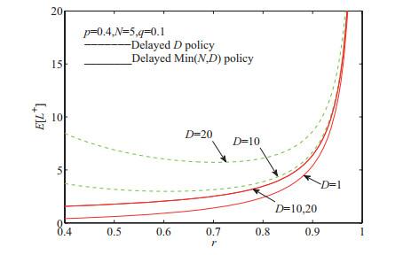
Figure 1 shows the average queue lengths

E [L^{+}]

for different values of

N

under varying

ρ

D

is fixed at

D = 20

. We see in Figure 1 that the average queue lengths under the delayed Min

(N, D)

-policy is smaller than or equal to those of the delayed

N

-policies because the average queue length is increasing with respect of

D

and the delayed Min(

N, \infty

)-policy is equivalent to the delayed

N

-policy. We note that

N = 1

implies the classical Geo/G/1 queueing system.

Figure 1 Comparison of the average queue length $E [L^{+}]$ for different values of $N$ and varying $ρ$

Full size|PPT slide

By varying

ρ

Figure 2 shows the average queue lengths for different values of

D

. We fixed the values of

p, q

and

N

p = 0.4, q = 0.1

and

N = 5

. We see in the figure that the mean queue lengths under the delayed Min

(N, D)

-policy is always smaller than those of the delayed

D

-policies. This is obvious if we consider the fact that the average queue length is an increasing function of

N

and that the delayed

D

-policy is equivalent to the delayed Min

(\infty, D)

-policy. The reason why the average queue lengths for

D = 10

and

D = 20

are almost the same is that for such large

D

, the system is controlled by

N

most of the time. We note that

D = 1

implies the classical M/G/1 queueing system.

Figure 2 Comparison of the average queue length $E [L^{+}]$ for different values of $D$ and varying $ρ$

Full size|PPT slide

Table 1 shows the steady state queue length distribution and the average queue length at epoch

n^{+}

for different values of

N

under the delayed

N

-policy and the delayed Min

(N, D)

-policy respectively. Here we select

p = 0.2, D = 20, μ = 2, q = 0.1

. When the parameter

D

is fixed at

D = 20

, we can see in table 1 that the steady state queue length distribution and the average queue length for

N = 20

and

N = 25

are almost the same under the delayed Min

(N, D)

-policy, which implies that for such large

N

, the effect of

N

on the system behavior is mere and the system is controlled by

D

. We note that such phenomena does not occur in Geo/G/1 queue with delayed

N

-policy. We note that

N = 1

implies the classical Geo/G/1 queueing system.

Table 1 The steady state queue length distribution and average queue length at epochs $n^{+}$ with parameters $p = 0.2, D = 20, μ = 2, q = 0.1$

$N$	1		3		5
d.p.	$N$	Min $(N, D)$	$N$	Min $(N, D)$	$N$	Min $(N, D)$
$p_{0}^{+}$	0.6	0.6	0.35	0.35	0.24706	0.24715
$p_{1}^{+}$	0.35	0.3	0.35	0.3	0.21176	0.21185
$p_{2}^{+}$	0.075	0.075	0.23125	0.23125	0.16324	0.16329
$p_{3}^{+}$	0.01875	0.01875	0.089063	0.089061	0.1511	0.15113
$p_{4}^{+}$	0.0046875	0.0046875	0.022266	0.022265	0.14807	0.14792
$p_{5}^{+}$	0.0011719	0.0011719	0.0055664	0.0055663	0.059076	0.058997
$p_{6}^{+}$	0.0002927	0.00029297	0.0013916	0.0013916	0.014769	0.014749
$p_{7}^{+}$	7.3242 $\times 10^{- 5}$	7.3242 $\times 10^{- 5}$	0.0003479	0.00034789	0.0036923	0.0036873
$p_{8}^{+}$	1.8311 $\times 10^{- 5}$	1.8311 $\times 10^{- 5}$	8.6975 $\times 10^{- 5}$	8.6973 $\times 10^{- 5}$	0.00092307	0.00092183
$p_{9}^{+}$	4.5776 $\times 10^{- 6}$	4.5776 $\times 10^{- 6}$	2.1744 $\times 10^{- 5}$	2.1743 $\times 10^{- 5}$	0.00023077	0.00023046
$p_{10}^{+}$	1.1444 $\times 10^{- 6}$	1.1444 $\times 10^{- 6}$	5.4359 $\times 10^{- 6}$	5.4358 $\times 10^{- 6}$	5.7692 $\times 10^{- 5}$	5.7615 $\times 10^{- 5}$
$E [L^{+}]$	0.5333	0.53333	0.1.1583	1.1583	2.0039	2.003

$N$	10		20		25
d.p.	$N$	Min $(N, D)$	$N$	Min $(N, D)$	$N$	Min $(N, D)$
$p_{0}^{+}$	0.14237	0.15042	0.077064	0.13659	0.062687	0.13659
$p_{1}^{+}$	0.12203	0.12893	0.066055	0.11707	0.053731	0.11707
$p_{2}^{+}$	0.094068	0.09938	0.050917	0.090242	0.041418	0.090242
$p_{3}^{+}$	0.087076	0.091975	0.047133	0.083518	0.03834	0.083518
$p_{4}^{+}$	0.085328	0.09002	0.046187	0.081743	0.03757	0.081743
$p_{5}^{+}$	0.084891	0.089109	0.046187	0.080916	0.037378	0.080916
$p_{6}^{+}$	0.084782	0.087591	0.045891	0.079537	0.037329	0.079537
$p_{7}^{+}$	0.084755	0.084133	0.045876	0.076397	0.037317	0.076397
$p_{8}^{+}$	0.084748	0.077411	0.045873	0.070293	0.037314	0.070293
$p_{9}^{+}$	0.084746	0.066696	0.045872	0.060563	0.037314	0.060563
$p_{10}^{+}$	0.033898	0.025755	0.045872	0.047777	0.037313	0.047777
$E [L^{+}]$	4.3469	4.0981	9.2489	4.7813	11.727	4.7813

Table 2 shows the steady state queue length distribution and the average queue length at epoch

n^{+}

for different values of

D

under the delayed

D

-policy and the delayed Min

(N, D)

-policy respectively. We fixed the values of

p = 0.25, μ = 2, q = 0.1

and

N = 4

. The reason why the steady state queue length distribution and the mean queue lengths for

D = 25

and

D = 30

are almost the same under the delayed Min

(N, D)

-policy is that for such large

D

, the system is almost controlled by the threshold value of

N

. Also, such phenomenon does not occur in Geo/G/1 queue with delayed

D

-policy. We note that

D = 1

implies the classical M/G/1 queueing system.

Table 2 The steady state queue length distribution and average queue length at epochs $n^{+}$ with parameters $p = 0.2, N = 4, μ = 2, q = 0.1$

$D$	1		5		10
d.p.	$D$	Min $(N, D)$	$D$	Min $(N, D)$	$D$	Min $(N, D)$
$p_{0}^{+}$	0.6	0.6	0.35	0.35462	0.23014	0.29532
$p_{1}^{+}$	0.3	0.3	0.29219	0.29604	0.1971	0.25293
$p_{2}^{+}$	0.075	0.075	0.18828	0.19077	0.15037	0.19296
$p_{3}^{+}$	0.01875	0.01875	0.10762	0.10904	0.13255	0.17009
$p_{4}^{+}$	0.0046875	0.0046875	0.044482	0.037154	0.11316	0.066522
$p_{5}^{+}$	0.0011719	0.0011719	0.013074	0.0092884	0.084717	0.01663
$p_{6}^{+}$	0.00029297	0.00029297	0.0032684	0.0023221	0.052322	0.0041576
$p_{7}^{+}$	7.3242 $\times 10^{- 5}$	7.3242 $\times 10^{- 5}$	0.00081711	0.00058053	0.025682	0.0010394
$p_{8}^{+}$	1.8311 $\times 10^{- 5}$	1.8311 $\times 10^{- 5}$	0.00020428	0.00014513	0.009872	0.00025985
$p_{9}^{+}$	4.5776 $\times 10^{- 6}$	4.5776 $\times 10^{- 6}$	5.1069 $\times 10^{- 5}$	3.6283 $\times 10^{- 5}$	0.009872	6.4963 $\times 10^{- 5}$
$p_{10}^{+}$	1.1444 $\times 10^{- 6}$	1.1444 $\times 10^{- 6}$	1.2767 $\times 10^{- 5}$	9.0707 $\times 10^{- 6}$	0.0007976	1.6241 $\times 10^{- 5}$
$E [L^{+}]$	0.53333	0.53333	1.2625	1.2193	2.3826	1.5335

$D$	20		25		30
d.p.	$D$	Min $(N, D)$	$D$	Min $(N, D)$	$D$	Min $(N, D)$ )
$p_{0}^{+}$	0.13659	0.28968	0.11351	0.28966	0.09711	0.28966
$p_{1}^{+}$	0.11707	0.24829	0.097297	0.24828	0.083237	0.24828
$p_{2}^{+}$	0.090242	0.19139	0.075	0.19138	0.064162	0.19138
$p_{3}^{+}$	0.083518	0.17713	0.069425	0.17715	0.059393	0.17715
$p_{4}^{+}$	0.081743	0.070136	0.068026	0.07015	0.058201	0.07015
$p_{5}^{+}$	0.080916	0.017534	0.06765	0.017538	0.057901	0.017538
$p_{6}^{+}$	0.079537	0.0043835	0.067446	0.0043844	0.057818	0.0043844
$p_{7}^{+}$	0.076397	0.0010959	0.067044	0.0010961	0.057765	0.0010961
$p_{8}^{+}$	0.070293	0.00027397	0.066026	0.00027402	0.057643	0.00027402
$p_{9}^{+}$	0.060563	6.8493 $\times 10^{- 5}$	0.063786	6.8506 $\times 10^{- 5}$	0.05731	6.8506 $\times 10^{- 5}$
$p_{10}^{+}$	0.047777	1.7123 $\times 10^{- 5}$	0.059622	1.7127 $\times 10^{- 5}$	0.05651	1.7127 $\times 10^{- 5}$
$E [L^{+}]$	4.7813	1.5677	6.0063	1.5678	7.2385	1.5678

Finally, under a special case, we further explain the importance of the steady state queue length distribution in the system capacity design.

In practice, the congestion of facilities is a key factor to be considered in decision-making process, since it has serious negative implications in both the manufacturing and the service sectors. The immediate consequence of congestion is that it leads to an increase in operating costs; further, the degradation in the quality of service results in customer dissatisfaction and eventual loss of market share. In most of the cases, queueing managers often use the stationary mean queue length to calculate the buffer capacity, so as to reduce the blocking probability of the system. However, through the following numerical example, we can see that employing the stationary mean queue length to estimate the buffer capacity may be not very suitable.

Let

p = 0.4, N = 5, D = 20, μ = 2, q = 0.1

, by Corollary 2, we obtain

E [L^{+}] = 3.562

. Furthermore, using the datums presented in Table 3, Equations (28) and (29) give the probability that the number of customers in the system exceeds the mean queue length. From the calculation results, we can realize that the probability of more than 30.833% is too high, this also means that a considerable number of customers will be rejected by the system due to no waiting place available upon arrival. Therefore, using the mean queue length to design the system capacity is quite inaccurate. On the other hand, from Table 3, we further observe that the probability that the number of customers in the system exceeds

24

is less than 0.01%. Thus, design a system with large capacity is also unnecessary. In practice, we may use the steady state queue length distribution and give some more reasonable system designs, so as to reduce the system operating costs.

\begin{aligned} P {L^{+} > E [L^{+}]} = 1 - \sum_{j = 0}^{E [L^{+}]} p_{j}^{+} = 1 - \sum_{j = 0}^{4} p_{j}^{+} = 0.30833, \end{aligned}

(28)

\begin{aligned} P {L^{+} > E [L^{+}] + 1} = 1 - \sum_{j = 0}^{E [L^{+}] + 1} p_{j}^{+} = 1 - \sum_{j = 0}^{5} p_{j}^{+} = 0.20555 . \end{aligned}

(29)

Table 3 The steady state queue length distribution at epochs $n^{+}$ with parameters $p = 0.4, N = 5, D = 20, μ = 2, q = 0.1$

$p_{0}^{+}$	$p_{1}^{+}$	$p_{2}^{+}$	$p_{3}^{+}$	$p_{4}^{+}$	$p_{5}^{+}$	$p_{6}^{+}$
0.10701	0.16594	0.1494	0.13836	0.13096	0.10278	0.068519
$p_{7}^{+}$	$p_{8}^{+}$	$p_{9}^{+}$	$p_{10}^{+}$	$p_{11}^{+}$	$p_{12}^{+}$	$p_{13}^{+}$
0.045679	0.030453	0.020302	0.013535	0.009023	0.0060153	0.0040102
$p_{14}^{+}$	$p_{15}$	$p_{16}^{+}$	$p_{17}^{+}$	$p_{18}^{+}$	$p_{19}^{+}$	$p_{20}^{+}$
0.0026735	0.0017823	0.0011882	0.00079214	0.0005281	0.00035206	0.00023471
$p_{21}^{+}$	$p_{22}^{+}$	$p_{23}^{+}$	$p_{24}^{+}$	$p_{25}^{+}$	$p_{26}^{+}$	$p_{27}^{+}$
0.00015647	0.00010432	6.9544 $\times 10^{- 5}$	4.6362 $\times 10^{- 5}$	3.0908 $\times 10^{- 5}$	2.0605 $\times 10^{- 5}$	1.3737 $\times 10^{- 5}$
$p_{28}^{+}$	$p_{29}^{+}$	$p_{30}^{+}$	$p_{31}^{+}$	$p_{32}^{+}$	$p_{33}^{+}$	$p_{34}^{+}$
9.158 $\times 10^{- 6}$	6.1053 $\times 10^{- 6}$	4.0702 $\times 10^{- 6}$	2.7135 $\times 10^{- 6}$	1.809 $\times 10^{- 6}$	1.206 $\times 10^{- 6}$	8.0399 $\times 10^{- 7}$
$p_{35}^{+}$	$p_{36}^{+}$	$p_{37}^{+}$	$p_{38}^{+}$	$p_{39}^{+}$	$p_{40}^{+}$	$p_{41}^{+}$
5.36 $\times 10^{- 7}$	3.5733 $\times 10^{- 7}$	2.3822 $\times 10^{- 7}$	1.5881 $\times 10^{- 7}$	1.0588 $\times 10^{- 7}$	7.0584 $\times 10^{- 8}$	4.7056 $\times 10^{- 8}$
$p_{42}^{+}$	$p_{43}^{+}$	$p_{44}^{+}$	$p_{45}^{+}$	$p_{46}^{+}$	$p_{47}^{+}$	$p_{48}^{+}$
3.1371 $\times 10^{- 8}$	2.0914 $\times 10^{- 8}$	1.3942 $\times 10^{- 8}$	9.295 $\times 10^{- 9}$	6.1967 $\times 10^{- 9}$	4.1311 $\times 10^{- 9}$	2.7541 $\times 10^{- 9}$

8 Conclusion

The research highlight of this work is the recursive formulae given by Theorems 5 to 8. They can be used to calculate the accurate numerical value of queue length distribution at different epochs

n^{-}, n

, and

n^{+}

. As far as we know, the recursive solution for queue length distributions at different time epochs are new. These performance measures can help us to make more accurate capacity planning decisions. Moreover, from Remark

2

we obtain the relations of queue length distribution among

p_{j}^{-}, p_{j}

and

p_{j}^{+}

References

Publishing order | Descend order by publishing year | Descend order by cited within

1	Yadin M, Naor P. Queueing systems with a removable service station. Operational Research Quarterly, 1963, 14, 393- 405. https://doi.org/10.1057/jors.1963.63 Cited in this article [1]

2	Balachandran K R. Control Policies for a single server system. Management Science, 1973, 19, 1013- 1018. https://doi.org/10.1287/mnsc.19.9.1013 Cited in this article [1]

3	Heyman D P. The $T$ -policy for the M/G/1 queue. Management Science, 1977, 23, 775- 778. https://doi.org/10.1287/mnsc.23.7.775 Cited in this article [1]

4	Levy H, Yechiali U. Utilization of idle time in an M/G/1 queueing system. Management Science, 1975, 22 (2): 202- 211. https://doi.org/10.1287/mnsc.22.2.202 Cited in this article [1]

5	Hur S, Paik S J. The effect of different arrival rates on the $N$ -policy of M/G/1 with server setup. Applied Mathematical Modelling, 1999, 23 (4): 289- 299. https://doi.org/10.1016/S0307-904X(98)10088-4 Cited in this article [1]

6	Wang K H, Huang K B. A maximum entropy approach for the $⟨ p, N ⟩$ -policy M/G/1 queue with a removable and unreliable server. Applied Mathematical Modelling, 2009, 33 (4): 2024- 2034. https://doi.org/10.1016/j.apm.2008.05.007 Cited in this article [1]

7	Tang Y H, Pu H, Yu M M. Queue size of M/G/1 queueing system with $N$ -policy and set-up times. Systems Engineering — Theory & Practice, 2011, 31 (1): 131- 137. Cited in this article [1]

8	Wei Y Y, Tang Y H, Gu J X. The queue length distribution and numerical calculation for Geo/G/1 queueing system with delayed $N$ -policy. Systems Engineering — Theory & Practice, 2011, 31 (11): 2151- 2160. Cited in this article [2]

Wei Y Y, Yu M M, Tang Y H, et al. Queue size distribution and capacity optimum design for

N

-policy Geo

. (λ_{1}, λ_{2}, λ_{3})

/G/1 queue with setup time and variable input rate. Mathematical and Computer Modelling, 2013, 57, 1559- 1571.

https://doi.org/10.1016/j.mcm.2012.12.032

Cited in this article [1]

10	Luo C Y, Tang Y H, Li W, et al. The recursive solution of queue length for Geo/G/1 queue with $N$ -policy. Journal of Systems Science and Complexity, 2012, 25 (2): 293- 302. https://doi.org/10.1007/s11424-012-9313-3 Cited in this article [1]

11	Lim D E, Lee D H, Yang W S, et al. Analysis of the GI/Geo/1 queue with $N$ -policy. Applied Mathematical Modelling, 2013, 37 (7): 4643- 4652. https://doi.org/10.1016/j.apm.2012.09.037 Cited in this article [1]

12	Chae K C, Park Y I. The queue length distribution for the M/G/1 queue under the $D$ -policy. Journal of Applied Probability, 2001, 38 (1): 278- 297. https://doi.org/10.1239/jap/996986663 Cited in this article [1]

13	Artalejo J R. On the M/G/1 queue with $D$ -policy. Applied Mathematical Modelling, 2001, 25 (12): 1055- 1069. https://doi.org/10.1016/S0307-904X(01)00031-2 Cited in this article [1]

14	Lee H W, Beak J W, Jeon J. Analysis of the M $. X$ /G/1 queue under $D$ -policy. Stochastic Analysis and Applications, 2005, 23 (4): 785- 808. https://doi.org/10.1081/SAP-200064479 Cited in this article [1]

15	Wang K H, Kuo C C, Ke J C. Optimal control of the $D$ -policy M/G/1 queueing system with server breakdowns. American Journal of Applied Sciences, 2008, 5 (5): 565- 573. https://doi.org/10.3844/ajassp.2008.565.573 Cited in this article [1]

16	Lee H W, Kim S A, Lee S W. Analysis and cost optimization of the M/G/1 queue under the $D$ -policy and LCFS discipline. Stochastic Analysis and Applications, 2008, 26 (1): 39- 59. Cited in this article [1]

17	Wei Y Y, Tang Y H, Gu J X. Queue size distribution and capacity optimum design for Geo/G/1 queueing system with delayed $D$ -policy. Systems Engineering — Theory & Practice, 2013, 33 (4): 996- 1005. Cited in this article [2]

18	Lee H W, Seo W J. The performance of the M/G/1 queue under the dyadic Min $(N, D)$ -policy and its cost optimization. Performance Evaluation, 2008, 65 (10): 742- 758. https://doi.org/10.1016/j.peva.2008.04.006 Cited in this article [1]

19	Lee H W, Seo W J, Lee S W, et al. Analysis of the MAP/G/1 queue under the Min $(N, D)$ -policy. Stochastic Models, 2010, 26 (1): 98- 123. https://doi.org/10.1080/15326340903517121 Cited in this article [1]

20	Tang Y H, Wu W Q, Liu Y P, et al. Queue length distribution of M/G/1 queueing system with Min $(N, V)$ -policy based on multiple server vacations. Systems Engineering — Theory & Practice, 2014, 34 (6): 1533- 1546. Cited in this article [1]

21	Hunter J J. Mathematical techniques of applied probability, Vol. Ⅱ, Discrete time models: Techniques and applications. New York: Academic Press, 1983. Cited in this article [1]

22	Bruneel H, Kim B G. Discrete-time models for communication systems including ATM. Boston: Kluwer Academic, 1993. Cited in this article [1]

23	Luo C Y, Tang Y H, Liu R B. Transient solution for queue-length distribution of Geometry/G/1 queueing model. Applied Mathematics — A Journal of Chinese Universities, Series B, 2007, 22 (1): 95- 100. https://doi.org/10.1007/s11766-007-0012-0 Cited in this article [3]

24	Jury E I. Theory and application of the $z$ -transform method. New York: John Wiley and Sons, 1964. Cited in this article [1]

Funding

the National Natural Science Foundation of China(71571127)

PDF(331 KB)

146

Accesses

Citation

Detail

Sections

Recommended

Abstract
Key words
Cite this article
1 Introduction
2 Model Formulation
3 Recursive Solution for Transient State Queue Length Distribution at Time Epoch $n^{+}$ During Server Busy Period
4 Solution for Transient State and Steady State Queue Length Distribution at Time Epoch $n^{+}$
5 Solution for Steady State Queue Length Distribution at Time Epochs $n^{-}$ and $n$
6 Several Special Cases
7 Numerical Examples and Discussion
Figure 1 Comparison of the average queue length $E [L^{+}]$ for different values of $N$ and varying $ρ$
Figure 2 Comparison of the average queue length $E [L^{+}]$ for different values of $D$ and varying $ρ$
Table 1 The steady state queue length distribution and average queue length at epochs $n^{+}$ with parameters $p = 0.2, D = 20, μ = 2, q = 0.1$
Table 2 The steady state queue length distribution and average queue length at epochs $n^{+}$ with parameters $p = 0.2, N = 4, μ = 2, q = 0.1$
Table 3 The steady state queue length distribution at epochs $n^{+}$ with parameters $p = 0.4, N = 5, D = 20, μ = 2, q = 0.1$
8 Conclusion
References
Funding

Received	Accepted	Published
2018-12-20	2019-03-29	2020-08-25
Issue Date
2020-08-25

Please choose a citation manager

Content to export

Abstract

Key words

Cite this article

1 Introduction

2 Model Formulation

3 Recursive Solution for Transient State Queue Length Distribution at Time Epoch $n^{+}$ During Server Busy Period

4 Solution for Transient State and Steady State Queue Length Distribution at Time Epoch $n^{+}$

5 Solution for Steady State Queue Length Distribution at Time Epochs $n^{-}$ and $n$

6 Several Special Cases

7 Numerical Examples and Discussion

Figure 1 Comparison of the average queue length $E [L^{+}]$ for different values of $N$ and varying $ρ$

Figure 2 Comparison of the average queue length $E [L^{+}]$ for different values of $D$ and varying $ρ$

Table 1 The steady state queue length distribution and average queue length at epochs $n^{+}$ with parameters $p = 0.2, D = 20, μ = 2, q = 0.1$

Table 2 The steady state queue length distribution and average queue length at epochs $n^{+}$ with parameters $p = 0.2, N = 4, μ = 2, q = 0.1$

Table 3 The steady state queue length distribution at epochs $n^{+}$ with parameters $p = 0.4, N = 5, D = 20, μ = 2, q = 0.1$

8 Conclusion

{{custom_sec.title}}

{{custom_sec.title}}

References

{{custom_fnGroup.title_en}}

Footnotes

Funding

Share

模态框（Modal）标题

Please choose a citation manager

Content to export

Abstract

Key words

Cite this article

1 Introduction

2 Model Formulation

3 Recursive Solution for Transient State Queue Length Distribution at Time Epoch n+ During Server Busy Period

4 Solution for Transient State and Steady State Queue Length Distribution at Time Epoch n+

5 Solution for Steady State Queue Length Distribution at Time Epochs n− and n

6 Several Special Cases

7 Numerical Examples and Discussion

Figure 1 Comparison of the average queue length E[L+] for different values of N and varying ρ

Figure 2 Comparison of the average queue length E[L+] for different values of D and varying ρ

Table 1 The steady state queue length distribution and average queue length at epochs n+ with parameters p=0.2,D=20,μ=2,q=0.1

Table 2 The steady state queue length distribution and average queue length at epochs n+ with parameters p=0.2,N=4,μ=2,q=0.1

Table 3 The steady state queue length distribution at epochs n+ with parameters p=0.4,N=5,D=20,μ=2,q=0.1

8 Conclusion

{{custom_sec.title}}

{{custom_sec.title}}

References

{{custom_fnGroup.title_en}}

Footnotes

Funding

3 Recursive Solution for Transient State Queue Length Distribution at Time Epoch $n^{+}$ During Server Busy Period

4 Solution for Transient State and Steady State Queue Length Distribution at Time Epoch $n^{+}$

5 Solution for Steady State Queue Length Distribution at Time Epochs $n^{-}$ and $n$

Figure 1 Comparison of the average queue length $E [L^{+}]$ for different values of $N$ and varying $ρ$

Figure 2 Comparison of the average queue length $E [L^{+}]$ for different values of $D$ and varying $ρ$

Table 1 The steady state queue length distribution and average queue length at epochs $n^{+}$ with parameters $p = 0.2, D = 20, μ = 2, q = 0.1$

Table 2 The steady state queue length distribution and average queue length at epochs $n^{+}$ with parameters $p = 0.2, N = 4, μ = 2, q = 0.1$

Table 3 The steady state queue length distribution at epochs $n^{+}$ with parameters $p = 0.4, N = 5, D = 20, μ = 2, q = 0.1$