Optimal Estimation for Power of Variance with Application to Gene-Set Testing

Min XIAO; Ting CHEN; Kunpeng HUANG; Ruixing MING

doi:10.21078/JSSI-2020-549-16

PDF(261 KB)

Journal of Systems Science and Information ›› 2020, Vol. 8 ›› Issue (6) : 549-564. DOI: 10.21078/JSSI-2020-549-16

Optimal Estimation for Power of Variance with Application to Gene-Set Testing

Author information +

History +

Abstract

Detecting differential expression of genes in genom research (e.g., 2019-nCoV) is not uncommon, due to the cost only small sample is employed to estimate a large number of variances (or their inverse) of variables simultaneously. However, the commonly used approaches perform unreliable. Borrowing information across different variables or priori information of variables, shrinkage estimation approaches are proposed and some optimal shrinkage estimators are obtained in the sense of asymptotic. In this paper, we focus on the setting of small sample and a likelihood-unbiased estimator for power of variances is given under the assumption that the variances are chi-squared distribution. Simulation reports show that the likelihood-unbiased estimators for variances and their inverse perform very well. In addition, application comparison and real data analysis indicate that the proposed estimator also works well.

Key words

high-dimensional diagonal covariance matrix / geometric shrinkage estimator / small sample / optimal shrinkage parameter / likelihood-unbiased estimator / hotelling's T² test

Cite this article

EndNote

Ris (Procite)

Bibtex

Download Citations

Min XIAO , Ting CHEN , Kunpeng HUANG , Ruixing MING. Optimal Estimation for Power of Variance with Application to Gene-Set Testing. Journal of Systems Science and Information, 2020, 8(6): 549-564 https://doi.org/10.21078/JSSI-2020-549-16

1 Introduction

Instead of working on a gene-by-gene basis, with the progress of biotechnology and other technologies, microarray technology can play an important role in addressing the issue of expression of thousands of genes from an experimental sample simultaneously^[1–3]. Biologists and medical scientists have also recognized that gene-set testing (e.g., judging where 2019 nCoV comes from by gene sequencing and testing) or pathway analysis is quite meaningful and necessary^{[4, 5]}. Due to the cost, the data available in public databases now contain mainly expression data ranging between 10, 000 and 55, 000 probe sets for fewer than 10 samples, e.g., the large amount of data generated by microarray technology is due mainly to the large number of genes represented on the array, rather than a large number of samples. While, for each gene the number of RNA samples assayed is typically small^[6]. In addition, it is not uncommon to see fewer than 10 subjects per tumor, e.g., Lönnstedt^[7], Kendziorski, et al.^[8], Dong, et al.^[9].

As a consequence, we are faced with a "large

p

, small

n

" paradigm, where "

p

" is the total number of genes and "

n

" is the number of replications. This problem is quite common in high-dimensional data. Therefore, the sample variances are inadmissible due to the relatively small number of replications and the commonly used statistical methods, such as

t

test or

F

test, for detecting differentially expressed genes on a gene-by-gene basis have low powers^[10]. Therefore, there is a growing body of literature that pay attention to the improvement of variance estimation of high-dimensional small sample data and its testing methods.

In terms of variance estimation, it is well known that improved variance estimation can substantially improve classification accuracy ^{[11, 12]} and power of testing differential gene expression for high dimensional low-sample-size data. Hence, in order to improve variance estimation, a variety of approaches: Bayesian estimators, Regression estimators and Shrinkage estimators are proposed. While, Bayesian method needs to determine the prior distribution and estimate its parameters, which is more complex. The Bayesian method can be referred to Kendziorski, et al.^[8], Smyth^[13], Fox and Dimmic^[14], Opgen-Rhein and Strimmer^[15], Hwang and Liu^[16] and Ji, et al.^[17]. About another method of variance estimation: Regression estimation, which including parametric and non-parametric methods, which is to apply the regression method to deal the variance increases proportionally with the intensity for microarray^[18]. But, the inconsistence of the estimate is a trouble. Specifically, it can be referred to Carroll and Wang^[19] and Wang, et al.^[20]. For the Shrinkage estimators, the idea originated from the James-Stein estimator of means^[21]. One of the earliest methods to stabilize the variance estimation was proposed by Tusher, et al.^[22]. In order to avoid the undue influence of the small variance estimates, he proposed to estimate the standard deviation

σ_{j}^{2}

(s_{j}^{2} + c) / 2

in their SAM test, where

c

is a constant acting as a shrinkage factor. Applying the standard James-Stein shrinkage method to log transformed estimates of variances, Cui, et al.^[6] proposed a James-Stein type shrinkage estimator for variances. Then, Tong and Wang^[23] and Tong, et al.^[24] derived a family of shrinkage estimators

{\hat{σ}}^{2 h}

and asymptotic properties for gene-specific variances raised to a fixed power

h

(nonzero) extending the idea from Cui, et al.^[6] to a more general setting under the Stein loss function:

L_{1} (σ^{2}, {\hat{σ}}^{2}) = {\hat{σ}}^{2} / σ^{2} - \ln ({\hat{σ}}^{2} / σ^{2}) - 1

and and the squared loss function:

L_{2} (σ^{2}, {\hat{σ}}^{2}) = {({\hat{σ}}^{2} / σ^{2} - 1)}^{2}

. These estimators borrow information across genes by shrinking each gene-specific variance estimator toward bias-corrected geometric mean of variance estimators for all genes. However, only iterative algorithm is given and have't explicit expression of shrinkage estimators for variances, at the same time, the calculation is intensive.

Therefore, there is a need to overcome these deficiencies. In this paper, under an new loss function:

L (W, \hat{W}) = ∥ \log \hat{W} - \log W ∥_{F}^{2}

(Arsigny, et al.^[25]), we propose a optimal geometric shrinkage estimation for power of variance based on the James-Stein estimator, which not only provides explicit expression for gene-specific variances, and calculate fastly also. As we know, computing speed is very important in processing high-dimensional data.

In the context of hypothesis testing, many tests modify the

t

test (or equivalently,

F

test) by shrinking the variances or the standard errors only are proposed in the earlier, for example, the SAM test^[22], the test of Wright and Simon^[26], the moderated

t

test ^[13] the multivariate MB-statistic^[27] and the

F_{S}

test^[6]. Later, Tong and Wang^[23] proposed a test similar to the

F_{S}

test and their idea has also been applied to discriminant analysis in Pang, et al.^[3]. The

F_{S}

test uses a shrinkage factor depending on the data, which seems more desirable. As we all known, the assumption that variances are equal for all genes is unlikely to be true. Contemporaneously, the optimal discovery procedure (ODP) proposed in Storey^[28] and Storey, et al.^[29] were shown to be much more powerful than above other procedures. However, it is very computationally intensive. Later, Hwang and Liu^[16] proposed a MAP tests in which the derive tests that maximize the average power with respect to some weight functions or prior distributions on the parameters and have more powerful than

F_{S}

test, but it needs shrinking both means and variances.

In recent years, a number of approaches to improve Hotelling's

T^{2}

test have emerged for testing high-dimensional data. In essence, with the main difference among them how the covariance matrix is handled, these approaches can be classified into the following three categories, the first category is the unscaled Hotelling's tests^{[4, 12]}. The covariance matrix is removed from Hotelling's

T^{2}

statistic to avoid the covariance matrix estimation. They demonstrated that the proposed test has better power than Hotelling's

T^{2}

test under the requirement of

p

and

n

being of the same order. The second category is the regularized Hotelling's tests^{[12, 30]}, which is applied to the covariance matrix estimation to resolve the singularity problem. The third category is the diagonal Hotelling's tests^[31–36]. In the third category, the covariance matrix is assumed to be diagonal. Under this assumption, the singularity problem is circumvented since a diagonal matrix is always invertible for non-zero entries, whether or not

p

is larger than

n

Here, we use the proposed optimal geometric shrinkage estimation for power of variance to construct the diagonal Hotelling's test statistics and compare with other 'information-sharing' statistics including the unscaled Hotelling's and regularized Hotelling's tests. It shows that the test statistics based on proposed shrinkage estimator have the highest or nearly the highest power.

The rest of the paper is organized as follows. First of all, in Section 2, we study how to obtain the geometric shrinkage estimator for power variance and give the relevant theorem. In Section 3, the performance of the proposed estimator is evaluated and compare it with some existing shrinkage estimators. Next, in Section 4, we show how to use geometric shrinkage estimator for power of variances to construct shrinkage-based diagonal Hotelling's tests statistics for tseting differential expression of genes with different forms of covariance and compare to some existing significant tests. Then, the application explanation is given by conducting a real data case in Section 5. Fianlly, we conclude in Section 6 with a brief discussion.

2 Geometric Shrinkage Estimate

Let

σ_{i}^{2}

be the variance of

X_{i}

i = 1, 2, \dots, p

. Assume each

X_{i}

is measured on

n

independent samples and denote

X_{k i}

as the

k

-th measurement on

X_{i}

k = 1, 2, \dots, n

and

i = 1, 2, \dots, p

. It is well known that, for each

i

σ_{i}^{2}

can be estimated by

s_{i}^{2} = (n - 1)^{- 1} \sum_{k = 1}^{n} (X_{k i} - \bar{X_{i}})^{2}

, where

\bar{X_{i}} = n^{- 1} \sum_{k = 1}^{n} X_{k i}

. Estimating

Σ^{h} = diag {σ_{1}^{2 h}, σ_{2}^{2 h}, \dots, σ_{p}^{2 h}}, h \neq 0

, a geometric shrinkage estimator is proposed by

\begin{array}{rcl} \hat{σ_{i}^{2 h}} = (c_{i 1} (h) t_{i}^{2 h})^{α} (c_{i 2} (h) s_{i}^{2 h})^{1 - α}, \end{array}

(1)

with some geometric shrinkage parameter

α \in [0, 1]

, where

t_{i}^{2}

is the target statistic,

c_{i 1} (h) > 0

c_{i 2} (h) > 0

are tuning parameters, which is chosen as follows:

c_{i 2} (h) s_{i}^{2 h}

is an unbiased estimator of

σ_{i}^{2 h}

, meanwhile

c_{i 1} (h) t_{i}^{2 h}

is an unbiased estimator of

σ^{2 h}

, where

σ^{2 h} = σ_{1}^{2 h} = \dots = σ_{p}^{2 h}

. We remark that two particular interesting cases in (2.1) are

h = 1

and

h = - 1

, which are the estimators of the variance and its inverse, respectively.

We assume that

(n - 1) s_{i}^{2} \sim σ_{i}^{2} χ^{2} (n - 1)

t_{i}^{2} = (\prod_{j = 1}^{p} s_{j}^{2})^{1 / p}

i = 1, 2, \dots, p

. It follows from ^[23] that, for any

0 \neq h > (1 - n) / 2

i = 1, 2, \dots, p

c_{i 1} (h) = (\frac{n - 1}{2})^{h} (\frac{Γ (\frac{n - 1}{2})}{Γ (\frac{n - 1}{2} + \frac{h}{p})})^{p}, c_{i 2} (h) = (\frac{n - 1}{2})^{h} \frac{Γ (\frac{n - 1}{2})}{Γ (\frac{n - 1}{2} + h)},

(2)

where

Γ (\cdot)

is the gamma function.

Under framework of Wald's statistical decision theory, the optimal geometric shrinkage parameter

α^{*}

is obtained by giving some loss function. In this paper, the loss function is chosen by

\begin{array}{rcl} L (W, \hat{W}) = ∥ l o g \hat{W} - l o g W ∥_{F}^{2} = \sum_{i = 1}^{p} (l o g ({\hat{w}}_{i}) - l o g (w_{i}))^{2}, \end{array}

(3)

where

W = diag (w_{1}, w_{2}, \dots, w_{p})

and its estimate

\hat{W} = diag ({\hat{w}}_{1}, {\hat{w}}_{2}, \dots, {\hat{w}}_{p})

are both positive definition matrices. Let

\begin{array}{rcl} \tilde{α} & = & arg min_{α} E (L (\hat{Σ^{h}}, Σ^{h})) \\ = & arg min_{α} \sum_{i = 1}^{p} E (α l o g c_{i 1} (h) t_{i}^{2 h} + (1 - α) l o g c_{i 2} (h) s_{i i}^{2 h} - l o g σ_{i}^{2 h})^{2} \\ = & \frac{\sum_{i = 1}^{p} E (l o g c_{i 2} (h) - l o g c_{i 1} (h) + h l o g s_{i}^{2} - h l o g t_{i}^{2}) (l o g c_{i 2} (h) + h l o g s_{i}^{2} - h l o g σ_{i}^{2})}{\sum_{i = 1}^{p} E (l o g c_{i 2} (h) - l o g c_{i 1} (h) + h l o g s_{i}^{2} - h l o g t_{i}^{2})^{2}} . \end{array}

(4)

Then, the optimal geometric shrinkage parameter is

\begin{array}{rcl} α^{*} = max {0, min {1, \tilde{α}}} . \end{array}

(5)

Remark 1 If

c_{i 1} (h) = c_{i 2} (h) \equiv 1

for all

i

and

h

, then (4) is

\begin{array}{rcl} \frac{\sum_{i = 1}^{p} E (l o g s_{i}^{2} - l o g t_{i}^{2}) (l o g s_{i}^{2} - l o g σ_{i}^{2})}{\sum_{i = 1}^{p} E (l o g s_{i}^{2} - l o g t_{i}^{2})^{2}}, \end{array}

(6)

which does not depend on

h

, so does

α^{*}

. In this case, the estimator of

σ_{i}^{2 h}

\begin{array}{rcl} \hat{σ_{i}^{2 h}} = (t_{i}^{2 h})^{α^{*}} (s_{i}^{2 h})^{1 - α^{*}} = (t_{i}^{2 α^{*}} s_{i}^{2 (1 - α^{*})})^{h} = (\hat{σ_{i}^{2}})^{h}, \end{array}

(7)

where

α^{*}

is the optimal geometric shrinkage parameter for

h = 1

Theorem 1 Assume that $(n - 1) s_{i}^{2} \sim σ_{i}^{2} χ^{2} (n - 1)$ , $t_{i}^{2} = (\prod_{j = 1}^{p} s_{j}^{2})^{1 / p}$ , $i = 1, 2, \dots, p$ . Then for any $0 \neq h > (1 - n) / 2$ , $i = 1, 2, \dots, p$ ,

\begin{array}{rcl} \tilde{α} = \frac{A}{B}, \end{array}

(8)

with

\begin{array}{rcl} A & = & p (\log c_{2} (h) - \log c_{1} (h)) \log c_{2} (h) + h^{2} (p - 1) ψ_{1} (\frac{n - 1}{2}) \\ + h p (\log c_{2} (h) - \log c_{1} (h)) (ψ_{0} (\frac{n - 1}{2}) - \log (\frac{n - 1}{2})) \end{array}

(9)

and

\begin{array}{rcl} B = p (l o g c_{2} (h) - l o g c_{1} (h))^{2} + h^{2} (p - 1) ψ_{1} (\frac{n - 1}{2}) + h^{2} \sum_{i = 1}^{p} [\log σ_{i}^{2} - \frac{1}{p} \sum_{j = 1}^{p} \log σ_{j}^{2}]^{2} . \end{array}

(10)

The likelihood-unbiased estimator of $\tilde{α}$ is

\begin{array}{rcl} \hat{\tilde{α}} = \frac{A}{\hat{B}} \end{array}

(11)

with

\begin{array}{rcl} \hat{B} = p (l o g c_{2} (h) - l o g c_{1} (h))^{2} + h^{2} (p - 1) ψ_{1} (\frac{n - 1}{2}) + h^{2} \sum_{i = 1}^{p} [\log s_{i}^{2} - \frac{1}{p} \sum_{j = 1}^{p} \log s_{j}^{2}]^{2} . \end{array}

(12)

3 Simulations

We compare the performance with Tong and Wang^[23] under two cases. Case 1 is

h = 1

, case 2 is

h = - 1

. We conduct simulations to evaluate the performance of the proposed geometric type shrinkage estimators

\hat{σ_{i}^{2}} (\hat{α_{opt 1}})

with

t_{i}^{2} = (\prod_{i = 1}^{p} s_{i}^{2})^{1 / p}

based on the percentage related improvement in average loss (PRIAL), which is defined as

\begin{array}{rcl} P R I A L = \frac{E (| | S - Σ | |_{F}^{2}) - E (| | \hat{Σ} - Σ | |_{F}^{2})}{E (| | S - Σ | |_{F}^{2})} \times 100, \end{array}

(13)

where

S = diag (s_{1}^{2}, s_{2}^{2}, \dots, s_{p}^{2})

and

\hat{Σ} = diag (\hat{σ_{1}^{2}}, \hat{σ_{2}^{2}}, \dots, \hat{σ_{p}^{2}})

are respective naive and proposed shrinkage estimators of

Σ = diag (σ_{1}^{2}, σ_{2}^{2}, \dots, σ_{p}^{2})

. A shrinkage estimator improves the naive estimator if its PRIAL is larger than

1

. We also compared the performance of the proposed geometric type shrinkage estimators with that of two estimators

\hat{σ_{i}^{2}} (\hat{α_{opt 2}})

and

\hat{σ_{i}^{2}} (\hat{α_{opt 3}})

proposed by Tong and Wang^[23]. Both of them assume

t_{i}^{2} = (\prod_{i = 1}^{p} s_{i}^{2})^{1 / p}

but the optimal shrinkage parameter

\hat{α_{opt 2}}

is obtained by minimizing the Stein loss function and

\hat{α_{opt 3}}

by minimizing the squared loss function. No explicit expression can be found for these optimal shrinkage parameters and a grid search method has to be used to obtain them under the classical asymptotic framework.

We set

p = 3000

and simulated 100 random samples of size

n = 6, 7, 8, 9, 10

from normal distributions. When the distribution of the sample is normal, in the

r

-th simulation, for a given sample size

n

, the true variance of each component of the sample was drawn from a Gamma distribution

gamma (α, β)

with specific shape parameter

α

and rate parameter

β

. That is, for each

(α, β)

, we first drew

p

observations

σ_{r 1}, \dots, σ_{r p}

from

gamma (α, β)

and then, for each

i

, randomly select

n

observations from

N (μ_{r i}, σ_{r i}^{2})

with

μ_{r i}

randomly drawn from

N (0, 1)

Gamma (1, σ_{r i}^{- 1 / 2})

. Denoted these observations by

X_{r i 1}, X_{r i 2}, \dots, X_{r i n}

. Four different shrinkage estimators

\hat{σ_{r i}^{2}} (\hat{α_{optk}})

k = 1, 2, 3

, as defined above, and naive estimator

s_{r i}^{2}

σ_{r i}^{2}

were then calculated from these observations. The final PRIAL of each shrinkage estimator is estimated by

\begin{array}{rcl} P R I A L_{k} = 100 \times (\frac{1}{100} \sum_{r = 1}^{100} \frac{\sum_{i = 1}^{p} (s_{r i}^{2} - σ_{r i}^{2})^{2} - \sum_{i = 1}^{p} (\hat{σ_{r i}^{2}} (\hat{α_{opt k}}) - σ_{r i}^{2})}{\sum_{i = 1}^{p} (s_{r i}^{2} - σ_{r i}^{2})^{2}}), \end{array}

(14)

where

k = 1, 2, 3

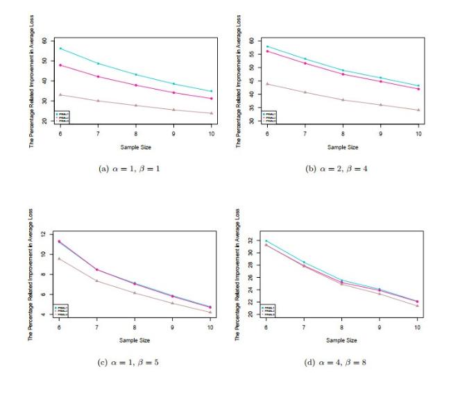
Figure 1 presents the plots of PRIAL against the sample size for the three estimators with the case

h = 1

considered in the simulations for four difference pairs of

(α, β) = (1, 1), (2, 4), (1, 5)

(4, 8)

when the gene expression levels are normally distributed. We can see from these figures that proposed shrinkage estimator has the largest improvement to the naive estimator for all sample sizes.

Figure 1 PRIALs of different estimators (1)

Full size|PPT slide

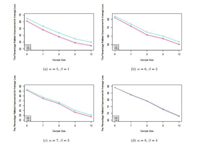
Figure 2 presents the plots of PRIAL against the sample size for the three estimators with the case

h = - 1

considered in the simulations for four difference pairs of

(α, β) = (5, 1), (6, 2), (7, 3), (8, 4)

when the gene expression levels are normally distributed. We can see from these figures that proposed shrinkage estimator has the largest improvement to the naive estimator for all sample sizes.

Figure 2 PRIALs of different estimators (2)

Full size|PPT slide

4 Application

In this section, we use the proposed estimator to construct the diagonal Hotelling's test for two-sample cases. According to Dong, et al.^[36], the shrinkage-based diagonal Hotelling's test for two-sample cases can be expressed as

T_{S D 2}^{2} ({\tilde{α}}^{*}) = \frac{n_{1} n_{2}}{n_{1} + n_{2}} {({\bar{X}}_{1} - {\bar{X}}_{2})}^{T} {\tilde{S}}_{p o o l}^{*} ({\bar{X}}_{1} - {\bar{X}}_{2}),

(15)

where

{\tilde{S}}_{p o o l}^{*} = diag {{\tilde{σ}}_{1, p o o l}^{- 2} ({\tilde{α}}^{*}), \dots, {\tilde{σ}}_{p, p o o l}^{- 2} ({\tilde{α}}^{*})}

. Note that, when

n_{1} + n_{2} > 6

, the chi-squared distribution (SDchi) can be used as a good approximate null distribution for small

p

. While, the normal distribution (SDnor) can be a good approximation for large

p

under the null hypothesis. The approximate null distributions are as follows, respectively,

T_{{S D}_{1}}^{2} ({\tilde{α}}^{*}) \sim N (ξ_{1}, τ_{1}), and T_{{S D}_{2}}^{2} ({\tilde{α}}^{*}) \sim c_{1} χ_{d_{1}}^{2}, as p \to \infty,

(16)

where

ξ_{1}

τ_{1}

are the mean and variance of normal distribution,

d_{1}

is the freedom of chi-squared distribution.

Under different scenarios of

p

and

n

, simulation comparison are performed with existing competitors which are unscaled Hotelling's test (CHEN)^[4], regularized Hotelling's test (RHT)^[12] and diagonal Hotelling's tests (PCT)^[31] and diagonal Hotelling's tests (SRI)^[34]. In addition, we analyze a gene expression data set to illustrate the shrinkage-based diagonal Hotelling's test under the proposed inverse estimator of variance.

4.1 Shrinkage-Based Diagonal Hotelling's Tests

In this subsection, we compare the shrinkage-based diagonal Hotelling's tests, including the chi-squared null distribution (SDchi) and the normal null distribution (SDnor), with some current methods in the aforementioned.

In our simulation, we generate data from the multivariate normal distribution with a common covariance matrix

Σ

to assess the type I error rate, the data are generated for both groups from

N_{p} (0, Σ)

. To assess the power, one group of data is generated from

N_{p} (0, Σ)

and the other one from

N_{p} (μ, Σ)

, where

μ_{j} = c σ_{j}^{2}

for

j = 1, 2, \dots, p

is randomly drawn from the scaled chi-squared distribution

(1 / 5) χ_{5}^{2}

The structure of the common covariance matrix is

Σ = D^{1 / 2} R D^{1 / 2}

, where

D = d i a g (Σ) = d i a g (σ_{1}^{2}, σ_{2}^{2}, \dots, σ_{p}^{2})

and

R

is the relation matrix. We use the following block-diagonal matrix as the correlation matrix:

\begin{array}{rcl} R = {(\begin{array}{ccccc} Σ_{ρ} & 0 & \dots & \dots & 0 \\ 0 & Σ_{- ρ} & 0 & ⋱ & ⋮ \\ ⋮ & 0 & Σ_{ρ} & 0 & ⋮ \\ ⋮ & ⋱ & 0 & Σ_{- ρ} & ⋱ \\ 0 & \dots & \dots & ⋱ & ⋱ \end{array})}_{p \times p}, \end{array}

(17)

where

Σ_{ρ}

is a

q \times q

matrix and

q \leq p

. We consider the following settings for

Σ_{ρ}

ρ = (σ_{i j})_{q \times q}

, where

σ_{i j} = ρ^{| i - j |}

for

1 \leq i, j \leq q

. Let

Σ_{A R}

denote this type of common covariance matrix. For

Σ_{A R}

, the correlation matrix is autoregressive of the order-1 structure. In our simulation, we set

n_{1} = n_{2} = n

from 5 to 60, and the effect sizes are

c = 0.52

and

0.3

. For different correlations, we set

ρ = 0, 0.3, 0.4 and 0.5

. The type I error rate and power are obtained by running 1000 simulations under the settings of

p = 60

q = 6

and

α = 0.05

, where

α

is the significance level. We first focus on the performances of all approaches for small sample sizes. The type I error rate and power are reported in Tables 1 and 2, respectively.

Table 1 Type I error rates for $p = 60$ under the null case

$ρ$	$Σ$	$n$	SDnor	SDchi	RHT	CHEN	SRI	PCT/wu
0	$Σ_{A R}$	5	0.042	0.0405	0.061	0	0.3712	0.173
		6	0.0395	0.047	0.078	0	0.2852	0.2172
		7	0.045	0.0435	0.064	0	0.2282	0.108
		8	0.04	0.0445	0.076	0	0.193	0.08
		9	0.0435	0.041	0.063	0	0.1584	0.062
		10	0.0435	0.05	0.063	0	0.1372	0.046
		60	0.0365	0.0486	0.053	0.086	0.0582	0.043
0.3	$Σ_{A R}$	5	0.047	0.0435	0.08	0	0.3504	0.1512
		6	0.046	0.0445	0.056	0	0.2618	0.1512
		7	0.046	0.0515	0.071	0	0.2092	0.097
		8	0.05	0.0445	0.056	0	0.1772	0.069
		9	0.048	0.049	0.063	0	0.1586	0.073
		10	0.0475	0.055	0.054	0	0.1414	0.056
		60	0.043	0.0495	0.053	0.073	0.0626	0.051
0.5	$Σ_{A R}$	5	0.0615	0.061	0.074	0	0.3046	0.25
		6	0.0645	0.0655	0.062	0	0.227	0.151
		7	0.0685	0.0655	0.07	0	0.177	0.088
		8	0.0655	0.071	0.067	0	0.158	0.073
		9	0.057	0.075	0.067	0	0.135	0.068
		10	0.067	0.0835	0.056	0	0.1214	0.065
		60	0.056	0.0805	0.055	0.047	0.0566	0.038

Table 2 Powers for $p = 60$ and $c = 0.52$ under the alternative case

$ρ$	$Σ$	$n$	SDnor	SDchi	RHT	CHEN	SRI	PCT/wu
0	$Σ_{A R}$	5	0.8845	0.734	0.804	0	0.995	0.855
		6	0.919	0.9165	0.934	0	0.997	0.973
		7	0.9865	0.9775	0.968	0	0.991	0.985
		8	0.9925	0.9905	0.954	0.005	0.997	0.982
		9	0.997	0.995	0.982	0.009	1	1
		10	1	1	0.99	0.11	0.999	1
		60	1	1	1	1	1	1
0.3	$Σ_{A R}$	5	0.8055	0.8175	0.812	0	0.957	0.964
		6	0.849	0.9825	0.946	0	0.954	0.959
		7	0.9585	0.981	0.948	0	0.994	0.914
		8	0.9935	0.993	0.938	0	0.996	0.982
		9	0.998	0.995	0.994	0.025	0.997	0.944
		10	0.9985	1	0.996	0.053	0.999	1
		60	1	1	1	1	1	1
0.5	$Σ_{A R}$	5	0.813	0.784	0.816	0	0.956	0.966
		6	0.936	0.878	0.888	0	0.957	0.936
		7	0.944	0.9415	0.934	0	0.984	0.915
		8	0.985	0.972	0.938	0	0.993	0.983
		9	0.997	0.999	0.988	0.013	0.999	0.992
		10	1	0.999	0.96	0.036	0.998	0.993
		60	1	1	1	1	1	1

From the results in Tables 1 and 2, we observe that the shrinkage-based diagonal Hotelling's tests outperform the other methods for different

ρ

. When the correlation is weak, our methods control the type I error rate well and at the same time maintain high power. As the correlation increases, the type I error rate of our methods becomes higher but it is still better than those of the other methods. PCT, SRI and RHT have high type I error rates when the sample size is smaller than 10. CHEN selects the null hypothesis too often and both of their powers are low. For higher correlations, these four approaches perform similarly.

In addition, we can see that diagonal Hotelling's tests, including our shrinkage-based methods, have the highest ROC curves. While, the unscaled Hotelling's test has the lowest ROC curves. This demonstrates that with limited numbers of observations, the diagonal Hotelling's tests are the best options.

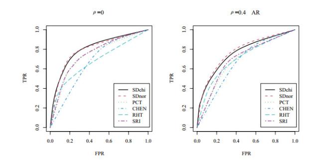
The superiority of the shrinkage-based diagonal Hotelling's tests is also demonstrated in Figure 3 and Table 3. Figure 3 shows the plots of the ROC curves and their respective AUC values are shown in Table 3. Here, we plot ROC curves with a range of FPR values from 0 to 1 and AUC values are also calculated in the same range as the FPR values. Without loss of generality, we plot the ROC curves for

n = 6

in Figure 3 to assess the overall performances of all approaches for small sample sizes. The figure shows that our methods, SDchi and SDnor, have the largest AUC values and highest ROC curves for all three correlations.

Figure 3 ROC curves for $n = 6$ , $p = 60$ and $c = 0.3$ . "AR" represents $Σ_{A R}$

Full size|PPT slide

Table 3 AUC values for $n = 6$ , $p = 60$ and $c = 0.3$

$ρ$	$Σ$	SDnor	SDchi	RHT	CHEN	SRI	PCT
0	$Σ_{A R}$	0.798	0.804	0.678	0.672	0.749	0.739
0.4	$Σ_{A R}$	0.776	0.761	0.704	0.668	0.698	0.687

4.2 Real Data Analysis

As we all know, the number of sample is small relative to the probe sets in many gene expression studies of cancer or tumor, and this phenomenon is not uncommon. This type of data is a typical high-dimensional small sample data. Therefore, we assess the performances of the shrinkage-based diagonal Hotelling's tests when they are applied to real gene expression data sets in this section. We studied the performance of each test statistical method in the test of glioma tumor data, which can be downloaded from GEO Data sets with accession number GDS1962.

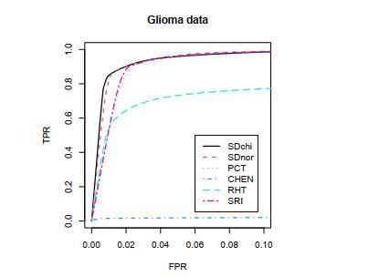
There are four classes of data in this data set: One non-tumor class and three glioma classes. Totally, the data include 54, 613 probes and 180 samples. We use the non-tumor (NON) class and the astrocytomas (AS) class, and the sample sizes are 23 and 26, respectively. Before using each test method, we randomly select 50 genes from genes, and then we use the test statistics in this paper to compare the advantages and disadvantages of each test statistics. In order to illustrate how the FPR and TPR are calculated, we use bootstrap method to select two groups from the non-tumor (NON) class to assess the type I errors. Instead, for the TPR, we use bootstrap method to take specitively a group from the non-tumor (NON) class oup and the astrocytomas (AS) class to assess the power. For each group, the number of samples is 5. The FPR and TPR are calculated based on 1000 simulations. Then, shows the ROC curves and AUC values are provided in Figure 4 and Table 4, Specifically.

Figure 4 ROC curves for Glioma data set when $p = 50$ and $n = 5$

Full size|PPT slide

Table 4 AUC values for $p = 50$ and $n = 5$

$D a t a s e t$	SDnor	SDchi	RHT	CHEN	SRI	PCT
Glioma	0.0892	0.0902	0.0648	0.0016	0.0852	0.0861

Similar to Figure 3, the ROC curves in Figure 4 are also generated with a range of FPR values from 0 to 0.1, and the same for AUC values. In Figure 4 and Table 4, our proposed estimations have the highest ROC curves and largest AUC values. That is, the diagonal Hotelling's tests used new estimetion perform better than the unscaled Hotelling's tests and the regularized Hotelling's tests when the sample size is small. This illustrates the advantage of the shrinkage-based diagonal Hotelling's tests compared with other test statistics in the case of small sample size and small copy number change at multiple probes.

5 Conclusion

In this paper, we consider the problem of variance estimation of high dimensional small sample population because sample variance is an unreliable variance estimator for limited observations, the optimal geometric shrinkage estimation for power of variance are proposed under a loss function that different from the previous. The estimation for power of variance not only has display expressions, but also is concise. Under the percentage related improvement in average loss (PRIAL), it performs better than the two estimators

\hat{σ_{i}^{2}} (\hat{α_{opt 2}})

and

\hat{σ_{i}^{2}} (\hat{α_{opt 3}})

proposed by Tong and Wang^[23]. Then, it can be well used to diagonal Hotelling's tests to test gene expression data, in addition, it has the advantage relation to the unscaled Hotelling's tests and the regularized Hotelling's tests when the sample size is small. Nevertheless, real data might come from heavy-tailed distributions or even discrete distributions, for example, RNA-seq data, which can obtained by next-generation sequencing technologies and have better coverage than microarray data, such data have already been applied in medical science. Then, the multivariate normal distribution is not a ideal choice to characterization these data. New methods need to be developed to analyze this data under new situation.

Acknowledgements

The authors gratefully acknowledge the Editor and two anonymous referees for their insightful comments and helpful suggestions that led to a marked improvement of the article.

Appendix

Proof Assume that

(n - 1) s_{i}^{2} \sim σ_{i}^{2} χ^{2} (n - 1)

t_{i}^{2} = (\prod_{j = 1}^{p} s_{j}^{2})^{1 / p}

i = 1, 2, \dots, p

. For any

0 \neq h > (1 - n) / 2

i = 1, 2, \dots, p

, we calculate the optimal shrinkage parameter as follows. First, note that

\begin{array}{rcl} E (\log (χ^{2} (n - 1))) = \log 2 + ψ_{0} (\frac{n - 1}{2}), \end{array}

(18)

and

\begin{array}{rcl} V a r (\log (χ^{2} (n - 1))) = ψ_{1} (\frac{n - 1}{2}), \end{array}

(19)

where

ψ_{0}

is the digamma function, and

ψ_{1}

is the trigamma function.

Second, when

t_{i}^{2} = (\prod_{j = 1}^{p} s_{j}^{2})^{1 / p}

, we show that

\begin{array}{rcl} \sum_{i = 1}^{p} E (l o g c_{2} (h) - l o g c_{1} (h) + h l o g s_{i}^{2} - h l o g t_{i}^{2}) (l o g c_{2} (h) + h l o g s_{i}^{2} - h l o g σ_{i}^{2}) \\ = & h^{2} (p - 1) ψ_{1} (\frac{n - 1}{2}) + h p (\log c_{2} (h) - \log c_{1} (h)) (ψ_{0} (\frac{n - 1}{2}) - \log (\frac{n - 1}{2})) \\ + p (\log c_{2} (h) - \log c_{1} (h)) \log c_{2} (h) . \end{array}

(20)

Write

\begin{array}{rcl} \sum_{i = 1}^{p} E (l o g c_{2} (h) - l o g c_{1} (h) + h l o g s_{i}^{2} - h l o g t_{i}^{2}) (l o g c_{2} (h) + h l o g s_{i}^{2} - h l o g σ_{i}^{2}) \\ = & \sum_{i = 1}^{p} (\log c_{2} (h) - \log c_{1 g} (h)) \log c_{2} (h) + h \sum_{i = 1}^{p} \log c_{2} (h) E (l o g s_{i}^{2} - l o g t_{i}^{2}) \\ + h \sum_{i = 1}^{p} (\log c_{2} (h) - \log c_{1} (h)) E (l o g s_{i}^{2} - l o g σ_{i}^{2}) + h^{2} \sum_{i = 1}^{p} E (l o g s_{i}^{2} - l o g t_{i}^{2}) (l o g s_{i}^{2} - l o g σ_{i}^{2}) \\ = & I + I I + I I I + I V . \end{array}

(21)

It is very easy to see that

\begin{array}{rcl} I = \sum_{i = 1}^{p} (\log c_{2} (h) - \log c_{1} (h)) \log c_{2} (h) = p (\log c_{2} (h) - \log c_{1} (h)) \log c_{2} (h), \end{array}

(22)

\begin{array}{rcl} I I = h \sum_{i = 1}^{p} \log c_{2} (h) E (l o g s_{i}^{2} - l o g t_{i}^{2}) = h \log c_{2} (h) \sum_{i = 1}^{p} E (l o g s_{i}^{2} - p^{- 1} \sum_{j = 1}^{p} l o g s_{j}^{2}) = 0. \end{array}

(23)

By (18) we have

\begin{array}{rcl} I I I & = & h \sum_{i = 1}^{p} (\log c_{2} (h) - \log c_{1} (h)) E (l o g s_{i}^{2} - l o g σ_{i}^{2}) \\ = & h (\log c_{2} (h) - \log c_{1} (h)) \sum_{i = 1}^{p} E (l o g χ_{i}^{2} (n - 1) - l o g (n - 1)) \\ = & h p (\log c_{2} (h) - \log c_{1} (h)) (ψ_{0} (\frac{n - 1}{2}) - \log (\frac{n - 1}{2})) . \end{array}

(24)

Now, we show that

\begin{array}{rcl} I V = h^{2} \sum_{i = 1}^{p} E (l o g s_{i}^{2} - l o g t_{i}^{2}) (l o g s_{i}^{2} - l o g σ_{i}^{2}) = h^{2} (p - 1) ψ_{1} (\frac{n - 1}{2}) . \end{array}

(25)

A similar argument yields

\begin{array}{rcl} \sum_{i = 1}^{p} E (l o g s_{i}^{2} - l o g t_{i}^{2}) (l o g s_{i}^{2} - l o g σ_{i}^{2}) \\ = & \sum_{i = 1}^{p} E (l o g χ_{i}^{2} (n - 1) - p^{- 1} \sum_{j = 1}^{p} l o g χ_{j}^{2} (n - 1) + \log σ_{i}^{2} - p^{- 1} \sum_{j = 1}^{p} l o g σ_{i}^{2} \\ \times (l o g χ_{i}^{2} (n - 1) - \log (n - 1)) \\ = & (1 - p^{- 1}) \sum_{i = 1}^{p} E (\log χ_{i}^{2} (n - 1))^{2} - p^{- 1} \sum_{i \neq j} E \log χ_{i}^{2} (n - 1) E \log χ_{j}^{2} (n - 1) \\ - \log (n - 1) \sum_{i = 1}^{p} (E l o g χ_{i}^{2} (n - 1) - p^{- 1} \sum_{j = 1}^{p} E l o g χ_{j}^{2} (n - 1)) \\ + \sum_{i = 1}^{p} (\log σ_{i}^{2} - p^{- 1} \sum_{j = 1}^{p} l o g σ_{i}^{2}) (E l o g χ_{i}^{2} (n - 1) - \log (n - 1)) \\ = & (p - 1) ψ_{1} (\frac{n - 1}{2}) . \end{array}

(26)

Thus, (25) holds. By (22)

\sim

(25) we arrival at (20). According to (23),

\begin{array}{rcl} \sum_{i = 1}^{p} E (l o g c_{2} (h) - l o g c_{1} (h) + h l o g s_{i}^{2} - h l o g t_{i}^{2})^{2} \\ = & \sum_{i = 1}^{p} (l o g c_{2} (h) - l o g c_{1} (h))^{2} + h (l o g c_{2} (h) \\ - l o g c_{1} (h)) E (l o g s_{i}^{2} - l o g t_{i}^{2}) + h^{2} \sum_{i = 1}^{p} E (l o g s_{i}^{2} - l o g t_{i}^{2})^{2} \\ = & \sum_{i = 1}^{p} (l o g c_{2} (h) - l o g c_{1} (h))^{2} + h^{2} \sum_{i = 1}^{p} E (l o g s_{i}^{2} - l o g t_{i}^{2})^{2} . \end{array}

(27)

By (26),

\begin{array}{rcl} \sum_{i = 1}^{p} E (l o g s_{i}^{2} - l o g t_{i}^{2})^{2} \\ = & \sum_{i = 1}^{p} E (l o g s_{i}^{2} - l o g t_{i}^{2}) (l o g s_{i}^{2} - l o g σ_{i}^{2}) + \sum_{i = 1}^{p} E (l o g s_{i}^{2} - l o g t_{i}^{2}) (l o g σ_{i} - l o g t_{i}^{2}) \\ = & (p - 1) ψ_{1} (\frac{n - 1}{2}) + \sum_{i = 1}^{p} E (l o g s_{i}^{2} - l o g t_{i}^{2}) l o g σ_{i}^{2} - \sum_{i = 1}^{p} E (l o g s_{i}^{2} - l o g t_{i}^{2}) l o g t_{i}^{2} \\ = & (p - 1) ψ_{1} (\frac{n - 1}{2}) + \sum_{i = 1}^{p} [\log σ_{i}^{2} - \frac{1}{p} \sum_{j = 1}^{p} \log σ_{j}^{2}]^{2} . \end{array}

(28)

Plugging (28) into (27), we have

\begin{array}{rcl} \sum_{i = 1}^{p} E (l o g c_{2} (h) - l o g c_{1} (h) + h l o g s_{i}^{2} - h l o g t_{i}^{2})^{2} \\ = & p (l o g c_{2} (h) - l o g c_{1} (h))^{2} + h^{2} (p - 1) ψ_{1} (\frac{n - 1}{2}) + h^{2} \sum_{i = 1}^{p} [\log σ_{i}^{2} - \frac{1}{p} \sum_{j = 1}^{p} \log σ_{j}^{2}]^{2} . \end{array}

(29)

Combining (21) and (29), we arrive at (8). It is well known that

s_{i}^{2}

is maximum the likelihood estimator of

σ_{i}^{2}

and,

(\log s_{i}^{2} - \frac{1}{p} \sum_{j = 1}^{p} \log s_{j}^{2})^{2}

is the maximum likelihood estimator of

(\log σ_{i}^{2} - \frac{1}{p} \sum_{j = 1}^{p} \log σ_{j}^{2})^{2}

by the "hereditary'' property of the maximum likelihood estimation. It follows from a well-known fact that a maximum likelihood estimator is likelihood-unbiased. Hence, (11) is the likelihood-unbiased estimator of (8).

References

Publishing order | Descend order by publishing year | Descend order by cited within

1	Efron B, Tibshirani R. On testing the significance of sets of genes. The Annals of Applied Statistics, 2007, 1(1): 107- 129. Cited in this article [1]

2	Newton M A, Quintana F A, Den Boon J A, et al. Random-set methods identify distinct aspects of the enrichment signal in gene-set analysis. The Annals of Applied Statistics, 2007, 1(1): 85- 106.

3	Pang H, Tong T J, Zhao H Y. Shrinkage-based diagonal discriminant analysis and its applications in high-dimensional data. Biometrics, 2009, 65(4): 1021- 1029. https://doi.org/10.1111/j.1541-0420.2009.01200.x Cited in this article [2]

4	Chen S X, Qin Y L. A two sample test for high dimensional data with applications to gene-set testing. Annals of Statistics, 2010, 38(2): 808- 835. Cited in this article [3]

5	Maciejewski H. Gene set analysis methods: Statistical models and methodological differences. Briefings in Bioinformatics, 2014, 15(4): 504- 518. https://doi.org/10.1093/bib/bbt002 Cited in this article [1]

6	Cui X Q, Hwang J T G, Qiu J, et al. Improved statistical tests for differential gene expression by shrinking variance components estimates. Biostatistics, 2005, 6(1): 59- 75. https://doi.org/10.1093/biostatistics/kxh018 Cited in this article [4]

7	Lönnstedt I, Speed T. Replicated microarray data. Statistica Sinica, 2001, 12(1): 31- 46. Cited in this article [1]

8	Kendziorski C, Newton M A, Lan H, et al. On parametric empirical bayes methods for comparing multiple groups using replicated gene expression profiles. Statistics in Medicine, 2003, 22(24): 3899- 3914. https://doi.org/10.1002/sim.1548 Cited in this article [2]

9	Dong S M, Nutt C L, Betensky R A, et al. Histology-based expression profiling yields novel prognostic markers in human glioblastoma. Journal of Neuropathology and Experimental Neurology, 2005, 64(11): 948- 955. https://doi.org/10.1097/01.jnen.0000186940.14779.90 Cited in this article [1]

10	Callow M J, Dudoit S, Gong E L, et al. Microarray expression profiling identifies genes with altered expression in hdl-deficient mice. Genome Research, 2000, 10(12): 2022- 2029. https://doi.org/10.1101/gr.147200 Cited in this article [1]

11	Maatta J M, Casella G. Developments in decision-theoretic variance estimation. Statistical Science, 1990, 5(1): 90- 101. Cited in this article [1]

12	Chen L S, Paul D, Prentice R L, et al. A regularized hotellings $t^{2}$ test for pathway analysis in proteomic studies. Journal of the American Statistical Association, 2011, 106(496): 1345- 1360. https://doi.org/10.1198/jasa.2011.ap10599 Cited in this article [4]

13	Smyth G K. Linear models and empirical bayes methods for assessing differential expression in microarray experiments. Statistical Applications in Genetics and Molecular Biology, 2004, 3(1): 1- 25. Cited in this article [2]

14	Fox R J, Dimmic M W. A two-sample bayesian $t$ -test for microarray data. BMC Bioinformatics, 2006, 7(1): 126- 126. https://doi.org/10.1186/1471-2105-7-126 Cited in this article [1]

15	Opgen-Rhein R, Strimmer K. Accurate ranking of differentially expressed genes by a distribution-free shrinkage approach. Statistical Applications in Genetics and Molecular Biology, 2007, 6(1): 1- 20. Cited in this article [1]

16	Hwang J T G, Liu P. Optimal tests shrinking both means and variances applicable to microarray data analysis. Statistical Applications in Genetics and Molecular Biology, 2010, 9(1): 1- 35. Cited in this article [2]

17	Ji T M, Liu P, Nettleton D. Borrowing information across genes and experiments for improved error variance estimation in microarray data analysis. Statistical Applications in Genetics and Molecular Biology, 2012, 11(3): 1- 29. Cited in this article [1]

18	Weng L, Dai H Y, Zhan Y H, et al. Rosetta error model for gene expression analysis. Bioinformatics, 2006, 22(9): 1111- 1121. https://doi.org/10.1093/bioinformatics/btl045 Cited in this article [1]

19	Carroll R J, Wang Y D. Nonparametric variance estimation in the analysis of microarray data: A measurement error approach. Biometrika, 2008, 95(2): 437- 449. https://doi.org/10.1093/biomet/asn017 Cited in this article [1]

20	Wang Y D, Ma Y Y, Carroll R J. Variance estimation in the analysis of microarray data. Journal of the Royal Statistical Society Series B — Statistical Methodology, 2009, 71(2): 425- 445. https://doi.org/10.1111/j.1467-9868.2008.00690.x Cited in this article [1]

21	James W, Stein C. Estimation with quadratic loss. Proceedings of the Fourth Berkeley Symposium on Mathematical Statistics and Probability, 1961, 1, 361- 379. Cited in this article [1]

22	Tusher V G, Tibshirani R, Chu G. Significance analysis of microarrays applied to the ionizing radiation response. Proceedings of the National Academy of Sciences of the United States of America, 2001, 98(9): 5116- 5121. https://doi.org/10.1073/pnas.091062498 Cited in this article [2]

23	Tong T J, Wang Y D. Optimal shrinkage estimation of variances with applications to microarray data analysis. Journal of the American Statistical Association, 2007, 102(477): 113- 122. https://doi.org/10.1198/016214506000001266 Cited in this article [6]

24	Tong T J, Jang H M, Wang Y D. James-stein type estimators of variances. Journal of Multivariate Analysis, 2012, 107, 232- 243. https://doi.org/10.1016/j.jmva.2012.01.019 Cited in this article [1]

25	Arsigny V, Fillard P, Pennec X, et al. Log-euclidean metrics for fast and simple calculus on diffusion tensors. Magnetic Resonance in Medicine, 2006, 56(2): 411- 421. https://doi.org/10.1002/mrm.20965 Cited in this article [1]

26	Wright G W, Simon R M. A random variance model for detection of differential gene expression in small microarray experiments. Bioinformatics, 2003, 19(18): 2448- 2455. https://doi.org/10.1093/bioinformatics/btg345 Cited in this article [1]

27	Tai Y C, Speed T P. A multivariate empirical bayes statistic for replicated microarray time course data. Annals of Statistics, 2006, 34(5): 2387- 2412. Cited in this article [1]

28	Storey J D. The optimal discovery procedure: A new approach to simultaneous significance testing. Journal of the Royal Statistical Society Series B — Statistical Methodology, 2007, 69(3): 347- 368. https://doi.org/10.1111/j.1467-9868.2007.005592.x Cited in this article [1]

29	Storey J D, Dai J Y, Leek J T. The optimal discovery procedure for large-scale significance testing, with applications to comparative microarray experiments. Biostatistics, 2007, 8(2): 414- 432. https://doi.org/10.1093/biostatistics/kxl019 Cited in this article [1]

30	Shen Y F, Lin Z Y, Zhu J. Shrinkage-based regularization tests for high-dimensional data with application to gene set analysis. Computational Statistics and Data Analysis, 2011, 55(7): 2221- 2233. https://doi.org/10.1016/j.csda.2010.12.013 Cited in this article [1]

31	Wu Y J, Genton M G, Stefanski L A. A multivariate two-sample mean test for small sample size and missing data. Biometrics, 2006, 62(3): 877- 885. https://doi.org/10.1111/j.1541-0420.2006.00533.x Cited in this article [2]

32	Srivastava M S, Du M. A test for the mean vector with fewer observations than the dimension. Journal of Multivariate Analysis, 2008, 99(3): 386- 402. https://doi.org/10.1016/j.jmva.2006.11.002

33	Srivastava M S. A test for the mean vector with fewer observations than the dimension under non-normality. Journal of Multivariate Analysis, 2009, 100(3): 518- 532. https://doi.org/10.1016/j.jmva.2008.06.006

34	Srivastava M S, Katayama S, Kano Y. A two sample test in high dimensional data. Journal of Multivariate Analysis, 2013, 114, 349- 358. https://doi.org/10.1016/j.jmva.2012.08.014 Cited in this article [1]

35	Park J Y, Ayyala D N. A test for the mean vector in large dimension and small samples. Quality Engineering, 2014, 59(1): 53- 54.

36	Dong K, Pang H, Tong T J, et al. Shrinkage-based diagonal hotelling's tests for high-dimensional small sample size data. Journal of Multivariate Analysis, 2016, 143, 127- 142. https://doi.org/10.1016/j.jmva.2015.08.022 Cited in this article [2]

Funding

the National Natural Science Foundation of China(11971433)

First Class Discipline of Zhejiang-A (Zhejiang Gongshang University- Statistics), Hunan Soft Science Research Project(2012ZK3064)

PDF(261 KB)

207

Accesses

Citation

Detail

Sections

Recommended

Received	Accepted	Published
2020-07-27	2020-09-09	2020-12-25
Issue Date
2020-12-25

Please choose a citation manager

Content to export

Abstract

Key words

Cite this article

1 Introduction

2 Geometric Shrinkage Estimate

3 Simulations

Figure 1 PRIALs of different estimators (1)

Figure 2 PRIALs of different estimators (2)

4 Application

4.1 Shrinkage-Based Diagonal Hotelling's Tests

Table 1 Type I error rates for $p = 60$ under the null case

Table 2 Powers for $p = 60$ and $c = 0.52$ under the alternative case

Figure 3 ROC curves for $n = 6$ , $p = 60$ and $c = 0.3$ . "AR" represents $Σ_{A R}$

Table 3 AUC values for $n = 6$ , $p = 60$ and $c = 0.3$

4.2 Real Data Analysis

Figure 4 ROC curves for Glioma data set when $p = 50$ and $n = 5$

Table 4 AUC values for $p = 50$ and $n = 5$

5 Conclusion

Acknowledgements

Appendix

{{custom_sec.title}}

{{custom_sec.title}}

References

{{custom_fnGroup.title_en}}

Footnotes

Funding

Share

模态框（Modal）标题

Please choose a citation manager

Content to export

Abstract

Key words

Cite this article

1 Introduction

2 Geometric Shrinkage Estimate

3 Simulations

Figure 1 PRIALs of different estimators (1)

Figure 2 PRIALs of different estimators (2)

4 Application

4.1 Shrinkage-Based Diagonal Hotelling's Tests

Table 1 Type I error rates for p=60 under the null case

Table 2 Powers for p=60 and c=0.52 under the alternative case

Figure 3 ROC curves for n=6, p=60 and c=0.3. "AR" represents ΣAR

Table 3 AUC values for n=6, p=60 and c=0.3

4.2 Real Data Analysis

Figure 4 ROC curves for Glioma data set when p=50 and n=5

Table 4 AUC values for p=50 and n=5

5 Conclusion

Acknowledgements

Appendix

{{custom_sec.title}}

{{custom_sec.title}}

References

{{custom_fnGroup.title_en}}

Footnotes

Funding

Table 1 Type I error rates for $p = 60$ under the null case

Table 2 Powers for $p = 60$ and $c = 0.52$ under the alternative case

Figure 3 ROC curves for $n = 6$ , $p = 60$ and $c = 0.3$ . "AR" represents $Σ_{A R}$

Table 3 AUC values for $n = 6$ , $p = 60$ and $c = 0.3$

Figure 4 ROC curves for Glioma data set when $p = 50$ and $n = 5$

Table 4 AUC values for $p = 50$ and $n = 5$