A Bounded Commitment in Vertical Collaborations of New Product Development

Zehui GE; Zhengkun REN; Qiying HU; Yiheng JIA

doi:10.21078/JSSI-2021-154-21

PDF(538 KB)

Journal of Systems Science and Information ›› 2021, Vol. 9 ›› Issue (2) : 154-174. DOI: 10.21078/JSSI-2021-154-21

A Bounded Commitment in Vertical Collaborations of New Product Development

Author information +

History +

Abstract

Uncertainty is a main source of opportunistic behaviors in research and development cooperations, which challenges strategic decisions ranging from investments to operations. To avoid opportunism arising in cooperations, commitments (either formal contracts or informal communications) are generally made in advance by members of an alliance. However, how does a commitment encourage R&D investments and ultimately enhance the total performance, without loss of flexibility in ex post operations? This study attempts to answer this by investigating a bounded commitment in the context of vertical collaborations in a supply chain. In this exploratory study, a 3-stage game model is used (by backward induction) to examine a two-echelon supply chain under a bounded commitment in NPD. Our analysis shows that upstream R&D investment is stimulated more and that both members are better off under the bounded commitment. At the same time, when the relative bargaining power between the supplier and the manufacturer falls into an appropriate area, it is possible to reach a bounded commitment, and the manufacturer is more sensitive to this relationship. Finally, the bounded commitment restrains opportunistic behaviors, but there is no strong sign that an increase in the ratio of the order outside the chain to the inside one can make firms better.

Key words

new product development / R&D cooperation / supply chain management / commitment / opportunistic behavior

Cite this article

EndNote

Ris (Procite)

Bibtex

Download Citations

Zehui GE , Zhengkun REN , Qiying HU , Yiheng JIA. A Bounded Commitment in Vertical Collaborations of New Product Development. Journal of Systems Science and Information, 2021, 9(2): 154-174 https://doi.org/10.21078/JSSI-2021-154-21

1 Introduction

Collaborating to research and develop new products is becoming unavoidable in firms' strategic decision-making, particularly in high-technology industries where digital tools used to facilitate distance collaboration. Managers generally prefer their business partners to competitors to cooperate in research and development (R & D), because a vertical relationship can exploit synergy and eliminate such conflicts arising in a horizontal relationship. However, effectively leveraging R & D efforts and innovative outputs requires careful consideration of uncertainty and opportunism in operations and productions. In practice, there remain some difficulties to overcome when trying to confirm such a long-run cooperative relationship by strategic commitments (either informal communications or formal contracts). Let us begin with two cases.

One case is a famous auto manufacturer (Denoted by F) in China and his partner (Denoted by C) in the United States. F began to cooperate with C in the 1980s. By 1986, F had developed a prototype of its new product based on a car model of C under the commitment that C would sell the complete production line to F. However, C held up the agreement when it saw a hot-selling in its domestic market. An extremely high price was proposed. But it never happened. The negotiations failed at the end of 1987 due to disagreements on the quotation price.

Another case is the cooperation between Dongfeng Motor (DFM) and Cummins Inc. that started in 1986. During their cooperation, they committed to keeping a long-term and steady partnership with each other. Importantly, they did so. More than 70% of Cummins engines (produced by their joint venture) were assembled into DFM's trucks, and the others were assembled into the non-DFM market but not DFM's direct competitors. In 2005, DFM and Cummins jointly established Cummins East Asia R & D Center, and they extended it in 2011. DFM accumulated not only fortune but also human resources and knowledge through the cooperation. Their R & D cooperation was not a one-man show of either Cummins or DFM; both of them participated deeply. According to BIS R & D scoreboard¹, DFM invested 2.3% of sales into R & D in 2010 with a 101% growth over average of last 4 years, and its rank climbed to 36th within the industry worldwide, and to 1st among Chinese auto makers. In 2013, Dongfeng planned to invest ＄2.5 billion in R & D over the next couple of years.

¹ http://webarchive.nationalarchives.gov.uk/20101208170217/;
http://www.innovation.gov.uk/rd_scoreboard/default.asp.

The two cases above have different cooperation paths and managerial senses for NPD collaborations in supply chain management (SCM). In the first case, F encountered its partner's holdup (a type of opportunistic behavior) due to a hot selling in the upstream (a type of uncertainty). The collaboration failed due to disagreements on the quotation price. In the second case, the upper stream (Cummins) made a commitment that the extra-chain sales of the components (i.e., engines) were limited at a certain level, uncertainty is considered in the commitment in advance. Moreover, their complementary R & D inputs significantly increased synergy, which has resisted corrosion of opportunistic behaviors.

There is seldom NPD collaboration free from challenges of opportunism². The typically uncertain nature of R & D activities makes it more difficult to disentangle non-compliance of partners from exogenous sources of failure of the R & D process and to write contracts contingent on R & D input to curb opportunism^[2]. In general, firms involved in NPD collaboration have to make some decisions carefully. For example, how can partners' opportunism be evaluated in such a long-run uncertain circumstance? In practice, many firms strategically commit something to each other to avoid a loss brought by opportunism. Then, how do they make a credible commitment? Does a commitment really promote R & D investments and enhance supply chain performance?

² According to [1], opportunism are those strategic non-cooperative self-interest-seeking behaviors with uncertainty.

In this paper, we want to answer the questions above by proposing a flexible commitment that depends on previous interactions in the framework of a supply chain consisting of a manufacturer and its supplier. The rest of the paper is organized as follows. We will review the related literature in the Section 2. The basic problem on our topic is described in Section 3, followed by a model and its analysis of the chain without any commitment in Section 3.2. We study the bounded commitment in Section 4. Finally, Section 5 concludes the paper.

2 Related Literature Review

This paper is related to three streams of existing literature.

The first stream examines vertical R & D cooperation for demand creation within a supply chain. According to [3], demand creation is one of the two main goals of R & D³. With regard to demand creation, most research on vertical NPD collaborations addresses partnership, cooperation patterns, and complementary drivers through empirical methods, e.g., [7, 8]. [9] offered a systematic review of IT usage in logistics and supply chain management to achieve a competitive advantage, where in such terms as collaborative innovation, flexibility, and value creation are addressed by the researchers. However, product development is an uncertain and long lead time activity with advance investments and collaboration between firms^[10]. Regarding collaborations in product development/design, [11] studied firms' investment in green product development, while [12] investigated product design such as final product design and quantity of new and remanufactured products, and their impact on closed-loop supply chain operations. Compared with no investment, [11] found that manufacturers investing in green product development is dominating in the long term. [13] found that both revenue sharing contract and linear quantity discount contract cannot fully coordinate the supply chain with demand disruptions. To eliminate potential risks, members in the alliance may under-invest in R & D in the absence of commitment. This phenomenon was noted by some researchers, e.g., [14, 15].

³ The other goal is cost reduction; see [4], [5] and [6] for examples.

The research on R & D collaboration within supply chains is an important but under-studied stream, although that on either cooperative R & D or SCM has made significant strides over the last two decades. Readers can see [16] and [17] for excellent reviews on SCM and R & D cooperation, respectively. Currently, the research on this stream is scattered across divergent topics and methods, e.g., [5, 7, 18, 19] etc. But the work most related to ours is [10], who examine two collaboration mechanisms observed in industrial practice: Sharing development costs and sharing development work. They show that the former is more attractive for new products with significant timing uncertainty, and this mechanism plays an important role in environments with uncertain product quality, similar capabilities across firms, and controllable cooperation costs.

On the basis of the above studies, this paper investigates how a certain commitment enlarges the investments in the context of R & D collaborations, focusing on firms' strategic commitments and flexibility in R & D investments (efforts).

The second stream of the literature examines commitments and opportunism in either R & D cooperation or supply chains. It consists of two topics.

First, evidence widely indicates that opportunism often exists in inter-firm relations^{[20, 21]}. [22] presented the drivers of opportunism from a contracting perspective; in a subsequent study, [23] proposed a conceptual framework to review the determinants of opportunism. [24] explored opportunistic behavior of purchasing professionals in strategic supplier relationships at the individual level, focusing on triggers, manifestations and consequences. However, as [25] noted, opportunistic behaviour erodes all members' long-term gains from cooperation. Moreover, [21] used an incomplete contracts approach to show that both anticipation and observability of opportunistic behaviour are typically not sufficient to prevent it when members can renegotiate contractual outcomes. Consequently, members of an alliance may under-invest in R & D to eliminate potential risks in the absence of commitment, a phenomenon highlighted by [14] and [15].

Second, as shown above, it is necessary for firms to make some commitments in such environment. Commitment refers to the willingness of partners to comply with the negotiated practices on behalf of the relationship^[26]. Research has also been conducted on bilateral commitment within supply chains. For example, [27] and [28] analyze order commitment as an operational strategy in supply chain management, and its mutual strategies from the partners, such as price discounts, demand forecast, etc. Along this direction, [29] investigated strategic commitment to a production schedule in a day-ahead electricity market, while [30] propose a commitment-based revenue-sharing and penalty model. [31] applied game theory to analyze suppliers' participation decision, identifying Bayesian Nash equilibrium strategies and characterize advantages of firm's commitment that may foster more innovativeness in the supply chain management. These studies investigate strategic commitments in production/operations, and show some basic and positive effects on supply chain performance.

Most of the literature above discusses supply or production contracts, with a few notable exceptions on vertical R & D collaboration. [14] considered a supplier's strategic commitment on price to stimulate downstream cost-reducing innovation. [32] demonstrated collaboration amongst the owners of the complementary producers with sectorwide commitments can be helpful in encouraging process innovation to support lean supply chains and sustainability. However, the supplier sacrifices an important means of responding to demand uncertainty once it makes a commitment. [33] studied collaborative cost reduction between two partners in a supply chain and propose an expected margin commitment to encourage the supplier to participate in this obviously profitable collaboration. By comparing this arrangement with a screening contract, they find that commitment is preferred when cost reduction is large or demand variability is low. [34] investigated a strategic commitment under cost uncertainty, and find that it encourages both firms' investments.

Based on the research above, we investigate commitments and efforts in demand-creating R & D when both members face uncertainty, including technological and demand uncertainty.

The third stream of the literature examines the flexibility of decision-making within supply chain. The flexibility of decision-making can often serve as an important buffer against market uncertainty or means of mitigating supply chain risks^{[35, 36]}. [37] investigated the role of allocation flexibility for achieving allocation flexibility against market demand uncertainty in supply chain, while [38] explored the value of the flexibility created by the transportation options in mitigating supply chain transportation risks. Some research focus on the effect of flexibility as an important role among the collaboration, commitment and production. [39] empirically examined the relationship between commitment and flexibility by analysing the benefits of commitment in terms of the integrated development of components and the flexibility provided by externally sourcing components. [40] extended the theory of supply chain flexibility by considering two types of flexibility, logistics flexibility and process flexibility, and examine how it is affected by such factors as demand, production, etc. It is followed by [41] who studied the design of process flexibility in a multiperiod production system. By investigating interactions between policy adjustments from governments and production decisions, [42] showed that a flexible subsidy policy is, on average, more expensive, unless there is a significant negative demand correlation across time periods. [43] explored the effect of supply chain flexibility and market agility and their role in SME performance, including responsiveness to customer needs and the speed of new product launches. However, the flexibility of commitments is seldom discussed in the field of vertical R & D collaborations.

In contrast to the research above, this paper will investigate how the flexibility benefit cooperation and output effectiveness within a supply chain.

3 The Basic Problem

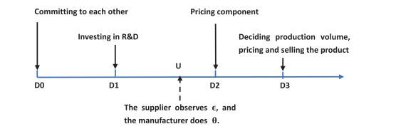
We investigate a simple supply chain with one manufacturer (denoted by "

m

") and one supplier (denoted by "

s

")⁴. They first commit some items to each other and then collaboratively invest in R & D. After this, the supplier produces and sells a new component to the manufacturer, and finally the manufacturer makes and sells a new product. More specifically, the supplier invests in R & D for a new component, and the manufacturer invests in R & D for the final product. The event sequence is described in the following and can be seen as a first look in Figure 1.

⁴ We adopt the convention of using the pronouns she and he to refer to the supplier and the manufacturer, respectively.

Figure 1 The event sequence of collaborative NPD with commitments

Full size|PPT slide

3.1 The Sequence of Events

We first specify their decision-making below, then present their commitments in Section 4.

D0: Committing to each other. The two firms commit some items to each other according to a certain committing rule. In this paper, we consider a rule that the supplier commits the wholesale price while the manufacturer commits the production volume. Although commitment can only be reached after several rounds of negotiation with each other, we emphasize commitment strategies and opportunistic behaviors other than the negotiation process in this paper. The content of the bounded commitment is in Section 4.

D1: Making R & D investments. In this stage, both firms simultaneously make their own R & D efforts (investments). In this paper, we adopt the "innovation level" to indicate R & D output. In the current literature, [44] define a concept of "innovation level", a scheme of non-subjective criteria for giving an award to innovative products and processes. For any given innovation level of the supplier, denoted by

x

, she has to make an R & D effort

u = u (x)

. Similarly, the manufacturer has to make an effort

v = v (y)

to achieve an innovation level

y

. As shown in the literature, more output requires more effort with an increasing marginal rate, i.e.,

u^{'} (x) > 0, v^{'} (y) > 0, u^{″} (x) > 0

and

v^{″} (y) > 0

The R & D output is measured by the new product's potential market, i.e.,

I = θ x y

, where the multiplicative relationship between

x

and

y

reflects a synergy effect, and

θ

is a random variable representing market uncertainty, to be described later. Let the corresponding efforts

u (x) = ρ x^{α}

and

v (y) = ρ y^{β}

with

ρ, α, β > 0

. [45] assumed linear costs of efforts in the analysis of the contract of collaborative services, with a parameter, denoting the marginal costs of efforts for both parties, In fact,

ρ

has a similar meaning here, but refers to marginal cost of innovation level. Similar assumptions can be found in the literature such as [46]. To simplify the model, we assume that the two firms are symmetrical in the R & D investment stage. Actually,

1 / α

and

1 / β

are the elasticities of

x

and

y

with respect to their own efforts. Then,

I = θ (u / ρ)^{1 / α} (v / ρ)^{1 / β}

, which satisfies a general form of the Cobb-Douglas production function. We also call

x

and

y

R & D efforts if there is no confusion because they have a 1-1 correspondence with

u

and

v

, respectively. Moreover, it is necessary to assume

1 / α + 1 / β < 1

to guarantee the strictly joint concavity of the chain profit. Otherwise, there may be no optimal R & D investment for the chain. As for

x^{α}

and

y^{β}

, quadratic functions are clearly unsuitable because

1 / α + 1 / β = 1

, although they are common in the literature.

This implies that the elasticity of output with respect to R & D effort (i.e.,

1 / α

1 / β

) will be significantly lower than 0.5 at the firm level (0.5 corresponds to the elasticity under quadratic functions). This has been demonstrated by the empirical research on R & D productivity. [47] reviewed the econometric literature on measuring the returns to R & D; they found that the R & D elasticity ranged from 0.01 to 0.25, but centered on 0.08 or so. More studies include [48] (ranging from 0.05 to 0.25) and [49] (ranging from 0.05 to 0.115 for OECD countries). Particularly, [50] studies the impact of the Internet on R & D efficiency and verifies that the Internet significantly improves R & D efficiency for high-tech firms, with an increase of 0.18 (from 0.12 to 0.30), but still less than 0.5.

These findings above support the view that the elasticity is far lower than 0.5. We therefore adopt biquadratic functions to model R & D efforts, that is,

u = ρ x^{4}

and

v = ρ y^{4}

. Actually, a new final product has to undergo two stages of inputs transformation: A transformation of R & D efforts into new technologies, and one of new technologies into a market potential. Each stage requires the concavity with respect to inputs, respectively. Thus, it is a biquadratic function of each firm's R & D effort, provided that a quadratic function was adopted in each stage. All functional forms introduced thus far are assumed to be common knowledge.

U: Observing information of uncertainties. After investments, the R & D output will be transferred into commercialized productions. Generally, the supplier may obtain some extra order by modifying the component and selling it with permission, and the manufacturer evaluates the future demand of the final product.

U1: Extra order of the supplier. As mentioned above, the supplier can get an extra order from other markets. For example, high-modularity components can be sold to other manufacturers with minor modifications. But it is not allowed to sell to other homogenous manufacturers, since the harm of this activity to the manufacturer has been confirmed by the literature [51, 52]. Denote the extra order by a random variable

ϵ

[\underline{ϵ}, \bar{ϵ}]

with mean

μ_{1}

and variance

σ_{1}^{2}

(i.e.,

E (ϵ) = μ_{1}

and

D (ϵ) = σ_{1}^{2}

), and the modifying cost is sufficiently low.

U2: Market uncertainty. As mentioned in

I = θ x y

, the potential market is also influenced by

θ

, a stochastic proxy of market uncertainty influenced by new technology and commercialization. As demonstrated by [53], project managers of NPD may have perceptions of such uncertainty regarding the application of technology to the current development project or regarding impending changes in that technology. So, we assume that the distribution of market uncertainty can be perceived by decision makers. Furthermore, let

θ

is distributed in

[\underline{θ}, \bar{θ}]

with mean

μ_{2}

and variance

σ_{2}^{2}

We assume that

ϵ

and

θ

are independent of each other, as shown in the introduction where the demand of engines from DFM's competitors is excluded by Cummins for the sake of a smooth cooperation. Our model is driven by the assumption that the market uncertainty, either of new components or of new products, is a public information. In other words, there is no private information; all firms can observe the values of both

ϵ

and

θ

once uncertainties are resolved. Unlike high confidentiality of firms' internal data, the market information can be accessed openly, to some extent, for firms within the supply chain, or calculated through some appropriate indicators, e.g., their capabilities, wholesale price of modified components, etc. Further, internet-based or digital tools now augment human thinking into analyzing more data efficiently, regarding communication and sharing of information directly within supply chains. Such information systems as ERP and S & OP (Sales and operations Planning) can serve to quickly and efficiently ensure that critical market information is communicated, or deduced from public sources (e.g., internet-based, or professional dataset). Particularly, advanced demand planning and proper strategies can also help uncover data and identify demand realized in partners'side.

D2: Pricing the component. We assume a wholesale price contract, simple but commonly observed^[54], under which the supplier decides a wholesale price

w

of new components, and its production pulled by the demand of new products. Extremely, the manufacturer can stop production and then clear new products when the demand is insufficient.

D3: Downstream production. As we know, it is difficult to precisely describe the dynamic of the demand because R & D collaboration is a long-lasting process with high uncertainty. In general, the manufacturer can forecast a rough, static demand before his decision-making, disregarding operational factors. Therefore, we assume the stock of new products can be cleared (i.e., the production volume

d

), and the market-clearing price is a function of

d

and

I

\begin{array}{rcl} p = I - k d = θ x y - k d, \end{array}

(1)

where

k

is constant which indicates a sensitive index of price to quantity.

3.2 The Chain Without Commitment

In this subsection, we investigate a three-stage game, i.e., Stage D1

\sim

D3, by ignoring the commitment stage D0.

By backward induction, we introduce the final stage first.

Stage D3: The manufacturer's production volume The manufacturer decides

d

in this stage, provided with R & D efforts

x

and

y

, the wholesale price

w

, and a realization of

θ

. Denote the unit production cost of the supplier and the manufacturer by

c_{s}

and

c_{m}

, respectively, and the total cost by

c = c_{s} + c_{m}

. Thus, the manufacturer's profit is

\begin{array}{rcl} π_{m} (d | x, y, w, θ) = (p - w - c_{m}) d - ρ y^{4}, \end{array}

(2)

where

p

satisfies Equation (1). For optimizing

π_{m}

above with respect to

d

, the optimal production is

\begin{array}{rcl} d^{*} (x, y, w, θ) = \arg max_{d} π_{m} (d | x, y, w, θ) = \frac{θ x y - w - c_{m}}{2 k} . \end{array}

(3)

Clearly the price is

p^{*} (x, y, θ) = θ x y - k d^{*} (x, y, w, θ) = (θ x y + w + c_{m}) / 2.

For convenience,

d^{*} (x, y, w, θ)

and

π_{m} (d | x, y, w, θ)

are written as

d^{*}

and

π_{m}

, respectively, and similarly to other notations below if there is no likelihood of confusion.

Stage D2: The supplier's wholesale pricing The supplier determines

w

to maximize her profit. Because the supplier cannot observe the realization of

θ

, her expected profit is in the following manner, provided with

x

y

, and revealing

ϵ

\begin{array}{rcl} π_{s} (w | x, y, ϵ) & = & E_{θ} [(w - c_{s}) (d^{*} + ϵ) - ρ x^{4}] \\ = & \frac{1}{2 k} (w - c_{s}) (μ_{2} x y - w - c_{m} + 2 k ϵ) - ρ x^{4}, \end{array}

(4)

where

E_{θ} [\cdot]

denotes the expectation with respect to

θ

Let

φ = μ_{2} x y - c

denote the expected unit-profit potential. The optimal price for maximizing

π_{s}

\begin{array}{rcl} w^{*} (x, y, ϵ) & = & c_{s} + \frac{φ}{2} + k ϵ . \end{array}

(5)

It is a separating equilibrium in the sub-game including Stage D2

\sim

D3.

Stage D1: Both firms' investments in NPD In this stage, the two firms play a Nash game in which they simultaneously decide their own R & D efforts. Substituting (5) into Equations (3) and (1), the production volume and retail price are, respectively,

\begin{array}{rcl} d^{*} (x, y, ϵ, θ) & = & \frac{φ}{4 k} + \frac{(θ - μ_{2}) x y}{2 k} - \frac{ϵ}{2}, \\ p^{*} (x, y, ϵ, θ) & = & c + \frac{3}{4} φ + \frac{(θ - μ_{2}) x y}{2} + \frac{k ϵ}{2} . \end{array}

Note that

E_{θ} (p) > c

if and only if

d < (μ_{2} x y - c) / k

, which means that the production is expected to be profitable only when the volume is lower than

(μ_{2} x y - c) / k

. Here,

(μ_{2} x y - c) / k

indicates a potential for a profitable production in the sense of expectation. As the innovation level increases, the bound becomes greater. Furthermore, as the value of

μ_{2}

increases, the bound becomes greater. Generally, the profitability of the new product has a positive effect on the supplier's extra profit. For instance, a high qualitative improvement of the new product makes it credible to promote the new component, even modified. Thus, we suppose

μ_{1}

is proportional to

(μ_{2} x y - c) / k

; that is,

μ_{1} = λ (μ_{2} x y - c) / k

for a certain positive constant

λ

. In details,

λ

indicates the ratio of the order outside the chain to the inside one, named the outside/inside (O/I) demand ratio in this paper. It makes sense to study a case in which the chain faces a positive production volume for all

(ϵ, θ)

, which also means

E_{ϵ} (E_{θ} (d^{*})) \geq 0

, i.e.,

λ \leq 1 / 2

. Otherwise, the chain will face a negative demand and then a negative profit.

As a support to the O/I demand ratio

λ

, we collect some data about the cooperation between Dongfeng and Cummins from DFM's annual reports and related articles. From their history of cooperation, we focus on the data from 1999 to 2005. The reason we eliminate the data after 2006 is that they established an R & D joint venture in 2006 and then developed multidimensional cooperation with other manufacturers, which may make the data lose purity in reflecting the specified cooperation. Table 1 gives an approximate representation of the ratio of Cummins' extra order from the non-DFM market to the sales volume of Dongfeng commercial vehicles (equipped by Cummins ISB & ISC series engines). Because it is so difficult to observe the potential demand of Dongfeng vehicles (i.e.,

(μ_{2} x y - c) / k

), we adopt the sales volume of Dongfeng commercial vehicles. Thus, the ratio can be approximately viewed as

λ

in this paper. From the ratio listed in the table, we can find

λ

kept in two stable areas:

0.110 \sim 0.14

0.273 \sim 0.335

. A higher level of

λ

in the later stage comes from two following facts. Before 2001, Cummins primarily sold ISB series to DFM and consequently increased the production of ISC. Another important fact is that the vehicle manufacturers faced a depressed market in China from 2002 to 2004, which certainly caused a stagnant demand of Dongfeng vehicles. The volume of ISB for non-DFM did not exceed 12.28% up to 2004, which was broken by Cummins' new strategy to enter the shipping industry in 2005.

Table 1 The ratio of Cummins' sales volume in non-Dongfeng market

Year	1999	2000	2001	2002	2003	2004	2005
CE	36600	-	-	114400	96300	122000	-
ND	3700	-	-	16000	13500	15000	-
DV	33100	-	-	47800	49500	45400	-
R	0.112	0.10	0.14	0.335*	0.273*	0.330*	0.28*

Remark: CE: Sales volume of Cummins engines; ND: CE in non-DFM; DV: Sales volume of Dongfeng vehicles equipped by Cummins; R: The ratio of ND to DV;
*: Including ISC series; -: Unnecessary.

Because there is no private information, the manufacturer can know about

ϵ

. For any given

x

y

, observations

ϵ

and

θ

, the two firms' profits are

\begin{array}{rcl} π_{s} (x, y, ϵ) = π_{s} (w^{*} | x, y, ϵ) = \frac{1}{2 k} (\frac{φ}{2} + k ϵ)^{2} - ρ x^{4}, \end{array}

(6)

\begin{array}{rcl} π_{m} (x, y, ϵ, θ) = π_{m} (d^{*} | x, y, w^{*}, θ) = \frac{1}{4 k} [\frac{φ}{2} + (θ - μ_{2}) x y - k ϵ]^{2} - ρ y^{4} . \end{array}

(7)

Thus, the two firms' expected profits in the R & D stage are,

\begin{array}{rcl} π_{s} (x, y) = E_{ϵ} [π_{s} (x, y, ϵ)] = \frac{φ^{2} (1 + 2 λ)^{2}}{8 k} + \frac{k σ_{1}^{2}}{2} - ρ x^{4}, \end{array}

(8)

\begin{array}{rcl} π_{m} (x, y) = E_{ϵ, θ} [π_{m} (x, y, ϵ, θ)] = \frac{1}{16 k} φ^{2} (1 - 2 λ)^{2} + \frac{σ_{2}^{2} x^{2} y^{2} + k^{2} σ_{1}^{2}}{4 k} - ρ y^{4}, \end{array}

(9)

respectively. Hence, the Nash game in Stage {D1} can now be written as

\begin{array}{rcl} {\begin{cases} max_{x} π_{s} (x, y), \\ max_{y} π_{m} (x, y) . \end{cases} \end{array}

(10)

Let

φ^{*} = μ_{2} x^{*} y^{*} - c

be the value of

φ

in equilibrium (see Theorem 2 in the appendix for equilibrium). Thus, the firms' profits in equilibrium are

\begin{array}{rcl} π_{s}^{*} & = & \frac{(1 + 2 λ)^{2}}{16 k} φ^{*} (φ^{*} - c) + \frac{k σ_{1}^{2}}{2}, \end{array}

(11)

\begin{array}{rcl} π_{m}^{*} & = & \frac{(1 - 2 λ)^{2}}{32 k} φ^{*} (φ^{*} - c) + \frac{σ_{2}^{2} (x^{*} y^{*})^{2} + 2 k^{2} σ_{1}^{2}}{8 k} . \end{array}

(12)

Both profits above consist of two parts:

● Mean profit, i.e., the first term, which represents the average level of the firm's profit;

● Opportunistic profit, the second term, which comes from opportunistic behavior. The opportunistic profit just relies on the realization of stochastic variables.

For example, the supplier's mean profit is

(1 + 2 λ)^{2} φ^{*} (φ^{*} - c) / (16 k)

, and her opportunistic profit is

k σ_{1}^{2} / 2

gained from a variation of

ϵ

. Recalling that the wholesale price

w^{*}

is uniquely determined by

ϵ

, and the supplier's profit is influenced by the variance of

ϵ

but is independent of that of

θ

. As a subsequent decision, the production volume of the manufacturer is determined by

w^{*}

and the realization of

θ

. Then, the variance of both

ϵ

and

θ

has an impact on the manufacturer's profit. Hence, the opportunistic profit of the supplier is only related to

σ_{1}

, but that of the manufacturer relates to both

σ_{1}

and

σ_{2}

Therefore, opportunistic behavior will appear in production and sales. [55] has verified that opportunism is unavoidable, especially in some extreme cases where its either a high extra demand of the new components or a very low potential demand of the final products may cause members deviations, even though some penalties may be imposed. For instance, the manufacturer will cut his order if the realization of

θ

is sufficiently low. However, this action may hurt the supplier, particularly when she faces a high setup cost. Similarly, when suppliers face higher external orders, i.e., the realization of

ϵ

, they can increase the wholesale price to obtain higher additional profits. But it is not easy for a partnering firm to engage in extremely aggressive forms of opportunistic behaviors. Under opportunistic behavior, the wholesale price of suppliers and the production volume of manufacturers will be adjusted within a range. If this is taken into account in the commitment formulation stage, whether it can improve the performance of the supply chain, we will study a flexible commitment in the next section.

4 Bounded Commitment

The commitments are made in Stage D0. Both firms first commit their own R & D investments

\tilde{x}

and

\tilde{y}

, simultaneously. Subsequently, the supplier commits an upper bound of wholesale price

\bar{w}

, followed by the manufacturer's commitment of the lower bound of production volume,

\underline{d}

In practice, the two firms have different half-open intervals for opportunistic behaviors, which has been verified by [55]. In details, the supplier commits an upper bound of the wholesale price while the manufacturer commits a lower one of the production volume. Compared with the commitment at a certain level, the bounded commitment allows the firm to justify its actions according to the circumstance. Clearly, the commitment on both the upper bound

\bar{w}

and the lower bound

\underline{d}

not only encourages flexibility, but also restrains themselves for a return from partners. Furthermore, the supplier generally expects an elevation of

\underline{d}

as a return when she drops

\bar{w}

. Thus, it is reasonable to assume

\underline{d}

reversely changes with

\bar{w}

. Consistent with Equation (3), we suppose that there is a linear relationship between

\bar{w}

and

\underline{d}

, in the following manner:

\begin{array}{rcl} \underline{d} = [μ_{2} x y - c - b (\bar{w} - c_{s})] / (2 k), \end{array}

(13)

where

b

is a exogenous coefficient reflecting a comparison between bargaining powers of the manufacturer and of the supplier in negotiations. In other words,

b

indicates a relative bargaining power between the manufacturer and the supplier. An increase in the bargaining power of the manufacturer will bring an increase in

b

. Inversely,

b

will decrease when the bargaining power of the supplier increases. Thus, the manufacturer will make a lower commitment of his production volume when the relative bargaining power

b

becomes a lower value. Exploiting Nash bargaining games, the literature has studied how barging powers affect the allocation of profit, e.g., [56, 57], and so on. Essentially, the relative bargaining power in this study directly affects the allocation of their profits in the alliance. From the perspective of supply chain management, [58] empirically investigate, and point out how the manufacturer margins are scaled by the factor

(1 - λ) / λ

where

λ

is the bargaining power of the downstream. The relative bargaining power

b

in our model is similar to the factor

(1 - λ) / λ

proposed by [58]. In particular, the equation above becomes (3) when

b = 1

Let us begin with Stage D3. Given

(\bar{w}, \underline{d})

and a realization of

(ϵ, θ)

, the manufacturer will optimize his profit function, the same with Equation (2), under the constraint

d \geq \underline{d}

. Thus, given

\tilde{x}

\tilde{y}

and

w

, the optimal production is

\begin{array}{rcl} \dot{d} & = & max {\frac{θ \tilde{x} \tilde{y} - w - c_{m}}{2 k}, \underline{d}} = {\begin{cases} \frac{θ \tilde{x} \tilde{y} - w - c_{m}}{2 k}, & if θ > θ^{'} := \frac{2 k \underline{d} + w + c_{m}}{\tilde{x} \tilde{y}}; \\ \underline{d}, & otherwise . \end{cases} \end{array}

(14)

Substituting it into Equation (4), the supplier's expected profit is

\begin{array}{rcl} π_{s} (w | \tilde{x}, \tilde{y}, \bar{w}, ϵ) & = & E_{θ} [(w - c_{s}) (\dot{d} + ϵ) - ρ {\tilde{x}}^{4}] \\ = & (w - c_{s}) [\int_{θ > θ^{'}} \frac{θ \tilde{x} \tilde{y} - w - c_{m}}{2 k} d F (θ) + \int_{θ \leq θ^{'}} \underline{d} d F (θ) + ϵ] - ρ {\tilde{x}}^{4} \\ = & \frac{w - c_{s}}{2 k} [μ_{2} \tilde{x} \tilde{y} - w - c_{m} + 2 k ϵ + \tilde{x} \tilde{y} \int_{\underline{θ}}^{θ^{'}} F (θ) d θ] - ρ {\tilde{x}}^{4}, \end{array}

(15)

where

F (\cdot)

is the distribution function of

θ

. The supplier will maximize her expected profit

π_{s} (w | \tilde{x}, \tilde{y}, \bar{w}, ϵ)

, subject to

w \leq \bar{w}

. Note that

π_{s} (w | \tilde{x}, \tilde{y}, \bar{w}, ϵ)

depends on

F (\cdot)

. Suppose that

θ

is uniformly distributed in

[\underline{θ}, \bar{θ}]

, so does

ϵ

[\underline{ϵ}, \bar{ϵ}]

. Furthermore, let

\bar{φ} = \bar{θ} \tilde{x} \tilde{y} - c

\underline{φ} = \underline{θ} \tilde{x} \tilde{y} - c

δ = \bar{ϵ} - \underline{ϵ}

and

Δ = (\bar{θ} - \underline{θ}) \tilde{x} \tilde{y}

. We have the following proposition.

Proposition 1 Given $ϵ$ and the committed bounds $\bar{w}$ and $\underline{d}$ , there is an optimal wholesale price $\dot{w}$ as follow:

\begin{array}{rcl} \dot{w} = {\begin{cases} c_{s} + \frac{2}{3} (\bar{φ} - 2 k \underline{d}) - \frac{1}{3} \sqrt{(\bar{φ} - 2 k \underline{d})^{2} - 12 k Δ (\underline{d} + ϵ)}, & i f ϵ \leq ϵ^{'}, \\ \bar{w}, & o t h e r w i s e, \end{cases} \end{array}

(16)

where $ϵ^{'}$ is a threshold uniquely determined by the following equation

\begin{array}{rcl} \bar{w} = c_{s} + {\begin{cases} \frac{Δ}{12} + \frac{2}{3} \tilde{φ} + \frac{4}{3} k ϵ^{'}, & i f b = 1 o r 3, \\ \frac{Δ (2 + b) - \sqrt{Δ^{2} (2 + b)^{2} - Δ (3 - 4 b + b^{2}) (Δ + 8 \tilde{φ} + 16 k ϵ^{'})}}{2 (3 - 4 b + b^{2})}, & o t h e r w i s e . \end{cases} \end{array}

(17)

The proposition above shows that

\dot{w}

is uniquely determined by

ϵ

and

ϵ^{'}

. Substituting Equations (16) and (17) into

π_{s} (w | \tilde{x}, \tilde{y}, \bar{w}, ϵ)

, the supplier's profit is

π_{s} (ϵ^{'} | \tilde{x}, \tilde{y}, ϵ) = \frac{1}{54 k Δ} {u^{3} + Φ [Φ^{2} + 36 k Δ (\underline{d} + ϵ)]} - ρ {\tilde{x}}^{4}

, where

Φ = \bar{φ} - 2 k \underline{d}

and

u = \sqrt{Φ^{2} - 12 k Δ (\underline{d} + ϵ)}

. Furthermore, the supplier's expected profit is

\begin{array}{rcl} π_{s} (ϵ^{'} | \tilde{x}, \tilde{y}) = E_{ϵ} π_{s} (ϵ^{'} | \tilde{x}, \tilde{y}, ϵ) = \frac{1}{δ} \int_{ϵ < ϵ^{'}} π_{s} (ϵ^{'} | \tilde{x}, \tilde{y}, ϵ) d ϵ + \frac{1}{δ} \int_{ϵ \geq ϵ^{'}} π_{s} (ϵ^{'} | \tilde{x}, \tilde{y}, ϵ) d ϵ . \end{array}

Because there is an 1-1 correspondence between

ϵ^{'}

and

\bar{w}

, it is equivalent to choose

ϵ^{'}

to maximize

π_{s} (ϵ^{'} | \tilde{x}, \tilde{y})

. Note that the two committed bounds are manufacturer commits a lower bound of production according to Equation (13). Thus, we have the following theorem.

Theorem 1 For $b \in [1, 3 / 2]$ , there must be a ceiling of $ϵ$ in $(μ_{1}, \bar{ϵ})$ , denoted by $ϵ^{'}$ such that it uniquely corresponds to the optimal price $\bar{w}$ , which is interior and above average.

The theorem is one of our significant findings in the sense that it ensures the existence of an interior point to commit. Otherwise, the setting of the ceiling at

ϵ^{'}

does not make sense for managers. We verify the existence of

\dot{w}

in bounded commitment in Proposition 1. According to Proposition 1 and Theorem 1, after the supplier observes the realization of

ϵ

, it can determine the optimal wholesale price according to the Equations (16) and (17). In fact, due to the constraint of the lower bound of the manufacturer's production volume, even if the supplier is facing high external market demand, it will not always increase the external chain orders, which restricts the opportunistic behavior that may occur in the supply chain.

Abbreviate

π_{s} (ϵ^{'} | \tilde{x}, \tilde{y})

π_{s} (\tilde{x}, \tilde{y})

for short, and denote the manufacturer's expected profit by

π_{m} (\tilde{x}, \tilde{y})

. Then,

\begin{array}{rcl} π_{m} (\tilde{x}, \tilde{y}) & = & \frac{1}{(\bar{θ} - \underline{θ}) δ} \int_{\underline{ϵ}}^{ϵ^{'}} [\int_{\underline{θ}}^{θ^{'}} π_{m} (\underline{d} | \tilde{x}, \tilde{y}, \dot{w}, θ) + \int_{θ^{'}}^{\bar{θ}} π_{m} (\dot{d} | \tilde{x}, \tilde{y}, \dot{w}, θ)] d θ d ϵ \\ + \frac{1}{(\bar{θ} - \underline{θ}) δ} \int_{ϵ^{'}}^{\bar{ϵ}} [\int_{\underline{θ}}^{θ^{'}} π_{m} (\underline{d} | \tilde{x}, \tilde{y}, \bar{w}, θ) + \int_{θ^{'}}^{\bar{θ}} π_{m} (\dot{d} | \tilde{x}, \tilde{y}, \bar{w}, θ)] d θ d ϵ \\ = & \frac{\tilde{x} \tilde{y}}{Δ δ} {\int_{\underline{ϵ}}^{ϵ^{'}} \int_{\underline{θ}}^{θ^{'}} [θ \tilde{x} \tilde{y} - \frac{μ_{2} \tilde{x} \tilde{y} - \bar{w} - c_{m}}{2} - \dot{w} - c_{m}] \frac{(μ_{2} \tilde{x} \tilde{y} - \bar{w} - c_{m})}{2 k} d θ d ϵ \\ + \int_{ϵ^{'}}^{\bar{ϵ}} \int_{\underline{θ}}^{μ_{2}} [\frac{(θ - μ_{2}) \tilde{x} \tilde{y} (μ_{2} \tilde{x} \tilde{y} - \bar{w} - c_{m})}{2 k} + \frac{(μ_{2} \tilde{x} \tilde{y} - \bar{w} - c_{m})^{2}}{4 k}] d θ d ϵ \\ + \int_{ϵ^{'}}^{\bar{ϵ}} \int_{μ_{2}}^{\bar{θ}} \frac{(θ \tilde{x} \tilde{y} - \bar{w} - c_{m})^{2}}{4 k} d θ d ϵ + \int_{\underline{ϵ}}^{ϵ^{'}} \int_{θ^{'}}^{\bar{θ}} \frac{(θ \tilde{x} \tilde{y} - \dot{w} - c_{m})^{2}}{4 k} d θ d ϵ} - ρ y^{4}, \end{array}

where

θ^{'} = max {\underline{θ}, μ_{2} - (\bar{w} - \dot{w}) / (\tilde{x} \tilde{y})}

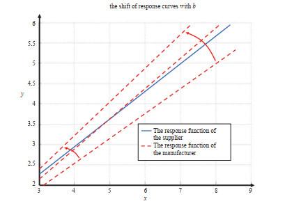
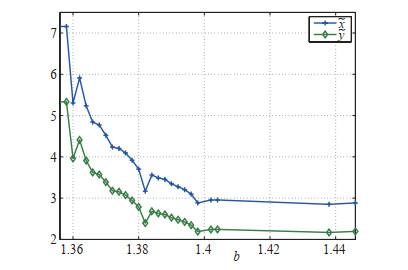
We investigate the equilibrium by numerical observations. Figure 2 shows a change in the response functions with

b

, in which

c_{s} = c_{m} = 50

k = 1

λ = 0.1

δ = 40

ρ = 6800

b \in [1.2, 1.5]

and

θ \sim U [240, 560]

. From the figure, we find that the manufacturer's response function changes along the arrows, whereas the supplier's scarcely moves, meaning that coefficient

b

has a significant effect on the manufacturer's response; i.e., the manufacturer exhibits a more sensitive response (with respect to

b

) than the supplier. However, we cannot simply state that the value of

b

has no effect on the supplier because it still influences the profit of the supplier through equilibrium. Through numerical analysis, we find that the existence of equilibrium just holds for a certain area of

b

. In other words, the equilibrium may not exist when

b

is extremely low or high, as shown in Figure 2 where

b

falls outside

[1.2, 1.5]

around. Moreover, the response function of the manufacturer moves upward with increase of

b

. From Figure 2, we can verify that the intersection of the two response functions moves towards the lower left quarter. In other words, both firms' investments generally decrease with

b

. This trend can be explicitly described by Figure 3.

Figure 2 The response curves change with $b$ when $b$ ranges in $[1.2, 1.5]$

Full size|PPT slide

Figure 3 The shift of equilibrium with $b$ when $b$ ranges in $[1.356, 1.446]$

Full size|PPT slide

In the bounded commitment, the investments decrease with

b

. Along this direction, the firms can set

b

as low as possible for larger profits and investments, but this action may challenge the existence of equilibrium. All in all, coefficient

b

in the bounded commitment plays a significant role in affecting the investments and profits. However, there is no sufficient evidence on how to determine

b

and who does it. A plausible interpretation lies in the fact that

b

appears in the collaboration as a parameter that may be influenced by, e.g., each member's power and techniques in negotiation. Furthermore, the bounded commitment needs a strong tie between members to achieve a suitable coefficient,

b

, which guarantees the existence of the equilibrium of investments. When

b

is larger, the greater the flexibility between the supplier's wholesale price and the manufacturer's production volume, it indicates that one party believes that the other party is more likely to deviate from the optimal situation without commitment (

b = 1

), so that they have reasons to reduce their investment level to avoid the other party take opportunistic behavior to bring more losses to themselves.

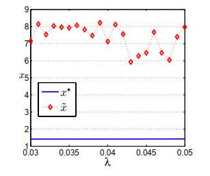
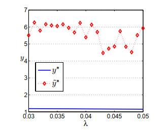
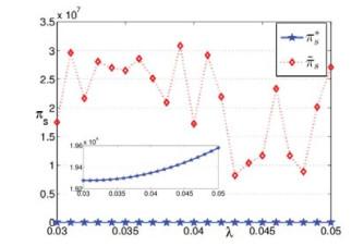
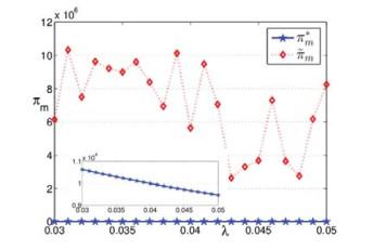
Figures 4 and 5 describe investment changes with

λ

x^{*}

and

y^{*}

without commitment,

\tilde{x}

and

\tilde{y}

under the bounded commitment when

b = 1.35

. Furthermore, Figures 6 and 7 compare the profits in which the sub-figures amplify slight variations in

π_{s}^{*}

and

π_{m}^{*}

. Similarly

x^{*}

and

y^{*}

have the same trends with

π_{s}^{*}

and

π_{m}^{*}

, respectively. The numerical comparison shows the dominance of the bounded commitment. Under the bounded commitment, the R & D investment level and profits of both firms increase significantly. We can also find that the supplier benefits from an increase in

λ

, it means the supplier can obtain more orders outside the chain, and inversely does the manufacturer when there is no commitment. This phenomenon is intuitive because the additional order of modified components primarily benefits the supplier, but it hurts the manufacturer because of externality.

Figure 4 The supplier's investment across different scenarios

Full size|PPT slide

Figure 5 The manufacturer's investment across different scenarios

Full size|PPT slide

Clearly, the commitment restrains opportunistic behaviors and then ties up members for a compatible pursuit of profit. Therefore, both firms benefit from the bounded commitment, but with a stable trend in general. In Figure 6 and 7, the high volatility may be caused by our numerical method in computing equilibrium, where a discrete method is adopted to find the intersection of both firms' response curves. However, we can still form a basic result from these figures above, that is, there is no strong sign that an increase in

λ

can make both firms (or either firm) better. A plausible explanation is that the bounded commitment brings a moderate flexibility and a weak constraint for members. Note that the bounded commitment coordinates the firms' decisions only when some extreme cases appear; otherwise, it gives them freedom in decision-making.

Figure 6 The supplier's profit across different scenarios

Full size|PPT slide

Figure 7 The manufacturer's profit across different scenarios

Full size|PPT slide

5 Conclusions

Opportunistic behavior appears to be a result of uncertainty in R & D cooperations, impeding strategic decisions in firms. Based on the literature review, we study R & D cooperation for demand creation within a supply chain and commitments and flexibility in either supply chains or R & D cooperation, respectively. In this paper, a bounded commitment was proposed in the framework of a supply chain consisting of a manufacturer and its supplier. This was to understand if commitments promote R & D investments and enhance supply chain performance as well as how an appropriate commitment can be made without loss of flexibility. We give a half-open interval bound of commitment with more flexibility. In doing so, we first identified the firms' decisions and incorporated a 3-stage game model (by backward induction) to examine them then later extended it to a bounded commitment where action dependent in NPD collaboration was proposed. We find that the bounded commitment can benefit both firms through bringing moderate flexibility for decision making and that commitment restrains opportunistic behaviors thus enhancing investments and increasing profits.

The main contribution of this paper is the investigation of the bounded commitment in vertical NPD collaboration with a focus on decision flexibility. R & D cooperation is a new topic appearing recently in supply chain management, though it has long been studied from the standpoint of R & D management. In the context of the interface between supply chain management and R & D cooperation, the research on flexible commitments is still in its infancy, particularly those under a demand-creative collaboration of NPD. In this paper, we verify the dominance of bounded commitments by quantitative analysis and numerical observation under a supply contract of wholesale price and a manufacturers commitment of production volume. Generally, the bounded commitment restrains opportunistic incentives, promote R & D investments, and then improve the whole supply chain performance.

Acknowledgements

The authors gratefully acknowledge the Editor and two anonymous referees for their insightful comments and helpful suggestions that led to a marked improvement of the article.

Appendix: proof of the theorems

Proof of Proposition 1

Let

t = w - c_{s}

, and rewrite

π_{s} (w | \tilde{x}, \tilde{y}, \bar{w}, ϵ)

π_{s} (t | \tilde{x}, \tilde{y}, \bar{w}, ϵ) = \frac{t}{2 k} [\tilde{φ} - t + 2 k ϵ + \frac{(2 k \underline{d} + t - \underline{φ})^{2}}{2 (\bar{φ} - \underline{φ})}] - ρ {\tilde{x}}^{4}

. Also, let

\frac{\partial}{\partial t} π_{s} (t | \tilde{x}, \tilde{y}, \bar{w}, ϵ) = 0

, then get

2 (\bar{φ} - \underline{φ}) (\hat{φ} - t + 2 k ϵ) - 2 t (\bar{φ} - 2 k \underline{d} - t) + (2 k \underline{d} + t - \underline{φ})^{2} = 0

, i.e.,

3 t^{2} - 4 (\bar{φ} - 2 k \underline{d}) t + 2 (\bar{φ} - \underline{φ}) (\tilde{φ} + 2 k ϵ) + (\underline{φ} - 2 k \underline{d})^{2} = 0

. Solving the quadratic equation of

t

yields the unique maximizer⁵ as

t = \frac{2}{3} (\bar{φ} - 2 k \underline{d}) - \frac{1}{3} \sqrt{(\bar{φ} - 2 k \underline{d})^{2} - 12 k (\underline{d} + ϵ) (\bar{φ} - \underline{φ})}

. This is exactly the case in Equation (16).

⁵ It can be examined that another solution of the equation does not satisfy the second-order optimality.

Now we turn to study

ϵ^{'}

. Denote

t^{'} = \bar{w} - c_{s}

. It is obvious that

lim_{ϵ \to ϵ^{'}} t = t^{'}

, i.e.,

\frac{2}{3} (\bar{φ} - 2 k \underline{d}) - \frac{1}{3} \sqrt{(\bar{φ} - 2 k \underline{d})^{2} - 12 k Δ (\underline{d} + ϵ^{'})} = t^{'}

. Substituting

\underline{d} = (\tilde{φ} - b t^{'}) / (2 k)

into it, we obtain

(3 - 4 b^{2} + b^{2}) t^{' 2} - Δ (2 + b) t^{'} + \frac{Δ^{2}}{4} + 2 Δ (\tilde{φ} + 2 k ϵ^{'}) = 0

. There are two cases in solving this equation of

t^{'}

. If

(3 - 4 b^{2} + b^{2}) = 0

(i.e.,

b = 1

b = 3

), then

t^{'} = \frac{Δ}{12} + \frac{2}{3} \tilde{φ} + \frac{4}{3} k ϵ^{'}

. Otherwise, we obtain two solutions:

t_{1, 2}^{'} = [Δ (2 + b) \pm \sqrt{Δ^{2} (2 + b)^{2} - Δ (3 - 4 b + b^{2}) (5 \bar{φ} + 3 \underline{φ} + 16 k ϵ^{'})}] / [2 (3 - 4 b + b^{2})]

. However, we can eliminate the greater one because

t^{'}

is not continuous at points

b = 1, 3

(actually

lim_{b \to 1, 3} t^{'} = \infty

). Thus, the proposition is proven.

Proof of Theorem 1

By accumulation,

π_{s} (ϵ^{'} | \tilde{x}, \tilde{y}) = E_{ϵ} π_{s} (ϵ^{'} | \tilde{x}, \tilde{y}, ϵ) = \frac{1}{δ} [\int_{ϵ < ϵ^{'}} + \int_{ϵ \geq ϵ^{'}}] π_{s} (ϵ^{'} | \tilde{x}, \tilde{y}, ϵ) d ϵ = \frac{{\bar{u}}^{5} - u^{' 5}}{1620 k^{2} Δ^{2} δ} + \frac{u^{' 3} (\bar{ϵ} - ϵ^{'})}{54 k Δ δ} + \frac{2 Φ}{3 δ} (\bar{ϵ} ϵ^{'} - \frac{ϵ^{' 2}}{2} - \frac{{\underline{ϵ}}^{2}}{2}) + \frac{Φ^{3}}{54 k Δ} + \frac{2}{3} \underline{d} Φ - ρ {\tilde{x}}^{4}

, where

\bar{u} = \sqrt{Φ^{2} - 12 k Δ (\underline{d} + \underline{ϵ})}

and

u^{'} = \sqrt{Φ^{2} - 12 k Δ (\underline{d} + ϵ^{'})}

. Similarly to the proof of Proposition 1, let

t^{'} = \bar{w} - c_{s}

. Then, we get

\begin{array}{rcl} \frac{\partial π_{s} (ϵ^{'} | \tilde{x}, \tilde{y})}{\partial ϵ^{'}} & = & [\frac{{\bar{u}}^{3} (Φ + 3 Δ) b}{324 k^{2} Δ^{2} δ} - \frac{u^{' 4} (2 b - 3)}{324 k^{2} Δ^{2} δ} + \frac{u^{' 2} (\bar{ϵ} - ϵ^{'}) (2 b - 3)}{18 k Δ δ}] \frac{d t^{'}}{d ϵ^{'}} + \frac{2 Φ (\bar{ϵ} - ϵ^{'})}{3 δ} \\ + [\frac{b (2 \bar{ϵ} ϵ^{'} - ϵ^{' 2} - {\underline{ϵ}}^{2})}{3 δ} + \frac{Φ^{2} b}{18 k Δ} - \frac{Φ b}{3 k} + \frac{2 \underline{d} b}{3}] \frac{d t^{'}}{d ϵ^{'}} - \frac{u^{' 3}}{54 k Δ δ} . \end{array}

(18)

Note that

t^{'}

is continuous when

b

approaches

1

. Thus, we just give the proof for

b \in (1, 3 / 2]

because the proof for

b = 1

can be similarly obtained as an extreme instance. From Equations (13), (16), and (17), we get

\begin{array}{rcl} {\begin{cases} Φ & = & \frac{Δ}{2} + b t^{'}, \\ u^{'} & = & Δ + (2 b - 3) t^{'}, \\ \frac{d t^{'}}{d ϵ^{'}} & = & \frac{4 k Δ}{\sqrt{Δ^{2} (2 + b)^{2} - Δ (3 - 4 b + b^{2}) (Δ + 8 \tilde{φ} + 16 k ϵ^{'})}} . \end{cases} \end{array}

(19)

Thus,

\frac{u^{' 3} (Φ + 3 Δ) b - u^{' 4} (2 b - 3)}{324 k^{2} Δ^{2} δ} \frac{d t^{'}}{d ϵ^{'}} = \frac{u^{' 3}}{54 k Δ δ}

. Denote

G (ϵ^{'}) = \frac{\partial π_{s} (ϵ^{'} | \tilde{x}, \tilde{y})}{\partial ϵ^{'}}

. Substitute them into Equation (18), then

G (ϵ^{'}) = [\frac{({\bar{u}}^{3} - u^{' 3}) (Φ + 3 Δ) b}{324 k^{2} Δ^{2} δ} + \frac{u^{' 2} (\bar{ϵ} - ϵ^{'}) (2 b - 3)}{18 k Δ δ} + \frac{b (2 \bar{ϵ} ϵ^{'} - ϵ^{' 2} - {\underline{ϵ}}^{2})}{3 δ}] \frac{d t^{'}}{d ϵ^{'}} + [\frac{Φ^{2} b}{18 k Δ} - \frac{Φ b}{3 k} + \frac{2 \underline{d} b}{3}] \frac{d t^{'}}{d ϵ^{'}} + \frac{2 Φ (\bar{ϵ} - ϵ^{'})}{3 δ}

. Therefore, it suffices to prove

G (μ_{1}) > 0

and

G (\bar{ϵ}) < 0

First,

G (μ_{1}) = [\frac{({\bar{u}}^{3} - u^{' 3}) (Φ + 3 Δ) b}{324 k^{2} Δ^{2} δ} + \frac{u^{' 2} (2 b - 3)}{36 k Δ} + \frac{b (4 \underline{d} + 3 μ_{1} + \underline{ϵ})}{6}] \frac{d t^{'}}{d ϵ^{'}} + (\frac{Φ^{2} b}{18 k Δ} - \frac{Φ b}{3 k}) \frac{d t^{'}}{d ϵ^{'}} + \frac{2 Φ}{3}

. Obviously,

\frac{d t^{'}}{d ϵ^{'}} \geq 0

. Thus, it suffices to prove

G (μ_{1}) \geq 0

when the coefficient of

\frac{d t^{'}}{d ϵ^{'}}

is negative. In Equation (19),

Δ^{2} (2 + b)^{2} - Δ (3 - 4 b + b^{2}) (Δ + 8 \tilde{φ} + 16 k ϵ^{'}) \geq Δ^{2} (2 + b)^{2} - 5 Δ^{2} (3 - 4 b + b^{2}) = Δ^{2} (- 11 + 24 b - 4 b^{2})

, where the inequality results from

2 \tilde{φ} \geq Δ

and

ϵ^{'} \geq 0

. Because

- 11 + 24 b - 4 b^{2} \geq 4 b^{2}

for

1 < b \leq \frac{3}{2}

\frac{d t^{'}}{d ϵ^{'}} \leq \frac{2 k}{b}

at the point

ϵ^{'} = μ_{1}

. When the coefficient of

\frac{d t^{'}}{d ϵ^{'}}

is negative, we have

G (μ_{1}) \geq \frac{({\bar{u}}^{3} - u^{' 3}) (Φ + 3 Δ)}{162 k Δ^{2} δ} + \frac{k (4 \underline{d} + 3 μ_{1} + \bar{ϵ})}{3} + \frac{Φ^{2}}{9 Δ} - \frac{u^{' 2} (3 - 2 b)}{18 b Δ}

by exploiting

\frac{d t^{'}}{d ϵ^{'}} \leq \frac{2 k}{b}

. Due to

Φ^{2} \geq u^{' 2}

, it is easy to prove

\frac{Φ^{2}}{9 Δ} \geq \frac{u^{' 2} (3 - 2 b)}{18 b Δ}

for

b \in (1, \frac{3}{2}]

. Furthermore,

{\bar{u}}^{3} \geq u^{' 3}

and

4 \underline{d} + 3 μ_{1} + \underline{ϵ} \geq 0

. Thus,

G (μ_{1}) \geq 0

holds.

Second,

G (\bar{ϵ}) = b [\frac{({\bar{u}}^{3} - u^{' 3}) (Φ + 3 Δ)}{324 k^{2} Δ^{2} δ} + \frac{2 (\underline{d} + μ_{1})}{3} + \frac{Φ^{2}}{18 k Δ} - \frac{Φ}{3 k}] \frac{d t^{'}}{d ϵ^{'}}

G (\bar{ϵ}) \leq 0

requires

\frac{({\bar{u}}^{3} - u^{' 3}) (Φ + 3 Δ)}{324 k^{2} Δ^{2} δ} + \frac{2 (\underline{d} + μ_{1})}{3} + \frac{Φ^{2}}{18 k Δ} - \frac{Φ}{3 k} \leq 0

. Recalling that Equation (16) indicates that

12 k Δ (\underline{d} + μ_{1}) \leq Φ^{2}

, i.e.,

\underline{d} + μ_{1} \leq Φ^{2} / (12 k Δ)

. Thus,

G (\bar{ϵ}) \leq 0

holds if

\begin{array}{rcl} \frac{({\bar{u}}^{3} - u^{' 3}) (Φ + 3 Δ)}{324 k^{2} Δ^{2} δ} + \frac{Φ^{2}}{9 k Δ} - \frac{Φ}{3 k} \leq 0. \end{array}

(20)

Equation (16) also indicates

\frac{Φ}{3} \leq t^{'} \leq \frac{2 Φ}{3}

. Combined with Equation (19),

\frac{Δ}{2 (3 - b)} \leq t^{'} \leq \frac{Δ}{(3 - 2 b)}

, then

0 \leq u^{'} \leq \frac{3 Δ}{2 (3 - b)}

and

\frac{3 Δ}{2 (3 - b)} \leq Φ \leq \frac{3 Δ}{2 (3 - 2 b)}

. Because

u^{3} - \frac{9 Δ}{4 (3 - b)} u^{2}

is decreasing in

u \in [0, \frac{3 Δ}{2 (3 - b)}]

{\bar{u}}^{3} - u^{' 3} \leq \frac{9 Δ}{4 (3 - b)} ({\bar{u}}^{2} - u^{' 2}) = \frac{27 k Δ^{2} δ}{3 - b}

for

ϵ^{'} = \bar{ϵ}

. Hence,

\frac{({\bar{u}}^{3} - u^{' 3}) (Φ + 3 Δ)}{324 k^{2} Δ^{2} δ} + \frac{Φ^{2}}{9 k Δ} - \frac{Φ}{3 k} \leq \frac{(Φ + 3 Δ)}{12 k (3 - b)} + \frac{Φ^{2}}{9 k Δ} - \frac{Φ}{3 k} = \frac{1}{36 k Δ (3 - b)} [4 (3 - b) Φ^{2} + 3 Δ (Φ + 3 Δ) - 12 (3 - b) Φ Δ]

. While,

4 (3 - b) Φ^{2} + 3 Δ (Φ + 3 Δ) - 12 (3 - b) Φ Δ = [2 (3 - b) Φ - 3 Δ] [2 Φ - \frac{3 Δ}{3 - 2 b}] - \frac{8 b^{2} - 28 b + 21}{3 - 2 b} Φ (3 Δ) - \frac{2 (b - 1)}{3 - 2 b} (3 Δ)^{2} \leq 0

for

Φ \in [\frac{3 Δ}{2 (3 - b)}, \frac{3 Δ}{2 (3 - 2 b)}]

and

b \in (1, \frac{3}{2}]

. Therefore, Equation (20) always holds, which means

G (\bar{ϵ}) \leq 0

Hence,

G (μ_{1}) \geq 0

and

G (\bar{ϵ}) \leq 0

. Clearly,

G (ϵ^{'})

is continuous. Thus, there must be an optimal solution in

[μ_{1}, \bar{ϵ}]

such that

G (ϵ^{'}) = 0

\bar{w} \geq \tilde{w}

can be obtained from the monotonicity of

\bar{w}

shown in Equation (19). Hence, the theorem is proven.

The existence of equilibrium without commitment

The following theorem gives the existence of equilibrium.

Theorem 2 There is a unique equilibrium $(x^{*}, y^{*}, w^{*}, d^{*})$ when $(1 + 2 λ)^{2} μ_{2}^{2} [μ_{2}^{2}$ $(1 - 2 λ)^{2} + 4 σ_{2}^{2}] > 512 k^{2} ρ^{2}$ .

Proof By Equation (8) and (9), we have

\frac{\partial}{\partial x} π_{s} (x, y) = \frac{φ}{4 k} μ_{2} y (1 + 2 λ)^{2} - 4 ρ x^{3}

\frac{\partial}{\partial y} π_{m} (x, y) = \frac{φ}{8 k} μ_{2} x (1 - 2 λ)^{2} + \frac{σ_{2}^{2} x^{2} y}{2 k} - 4 ρ y^{3}

. Let them be zero, then any equilibrium must satisfy the first-order conditions:

\begin{array}{rcl} {\begin{cases} (μ_{2} x y - c) μ_{2} x y (1 + 2 λ)^{2} = 16 k ρ x^{4}, \\ (μ_{2} x y - c) μ_{2} x y (1 - 2 λ)^{2} + 4 σ_{2}^{2} x^{2} y^{2} = 32 k ρ y^{4} . \end{cases} \end{array}

(21)

Multiplying the two equations yields

(1 + 2 λ)^{2} μ_{2} (μ_{2} x y - c) [(μ_{2} x y - c) μ_{2} (1 - 2 λ)^{2} + 4 σ_{2}^{2} x y] = 512 k^{2} ρ^{2} (x y)^{2}

. This is a quadratic equation for

x y

. By solving the equation, we get two roots as follows:

\begin{array}{rcl} x^{*} y^{*} = c μ_{2} \frac{(1 + 2 λ)^{2} [μ_{2}^{2} (1 - 2 λ)^{2} + 2 σ_{2}^{2}] \pm 2 (1 + 2 λ) \sqrt{128 (1 - 2 λ)^{2} k^{2} ρ^{2} + (1 + 2 λ)^{2} σ_{2}^{4}}}{(1 + 2 λ)^{2} μ_{2}^{2} [μ_{2}^{2} (1 - 2 λ)^{2} + 4 σ_{2}^{2}] - 512 k^{2} ρ^{2}} . \end{array}

Under the condition

(1 + 2 λ)^{2} μ_{2}^{2} [μ_{2}^{2} (1 - 2 λ)^{2} + 4 σ^{2}] > 512 k^{2} ρ^{2}

, the smaller root would bring a negative margin of the new product, i.e.,

μ_{2} x^{*} y^{*} - c < 0

. Therefore, it is omitted.

Dividing the second equation by the first one of (21), we get

\frac{(1 - 2 λ)^{2}}{(1 + 2 λ)^{2}} = \frac{32 k ρ y^{4} - 4 σ_{2}^{2} x^{2} y^{2}}{16 k ρ x^{4}} = 2 (\frac{y}{x})^{4} - \frac{σ_{2}^{2}}{4 k ρ} (\frac{y}{x})^{2}

, which can be viewed as a quadratic equation of

(x / y)^{2}

. By rearranging terms, we get the unique non-negative root as

\begin{array}{rcl} {(\frac{x^{*}}{y^{*}})}^{2} = (1 + 2 λ) \frac{\sqrt{128 k^{2} ρ^{2} (1 - 2 λ)^{2} + (1 + 2 λ)^{2} σ_{2}^{4}} - (1 + 2 λ) σ_{2}^{2}}{8 k ρ (1 - 2 λ)^{2}} . \end{array}

Therefore,

x, y

is uniquely determined by the following two equations:

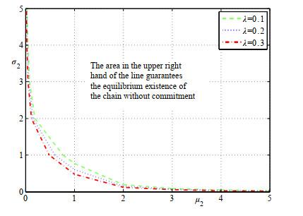
\begin{array}{rcl} {\begin{cases} x^{*} y^{*} = c μ_{2} \frac{(1 + 2 λ)^{2} [μ_{2}^{2} (1 - 2 λ)^{2} + 2 σ_{2}^{2}] + 2 (1 + 2 λ) \sqrt{128 (1 - 2 λ)^{2} k^{2} ρ^{2} + (1 + 2 λ)^{2} σ_{2}^{4}}}{(1 + 2 λ)^{2} μ_{2}^{2} [μ_{2}^{2} (1 - 2 λ)^{2} + 4 σ_{2}^{2}] - 512 k^{2} ρ^{2}}, \\ (x^{*} / y^{*})^{2} = (1 + 2 λ) \frac{\sqrt{128 k^{2} ρ^{2} (1 - 2 λ)^{2} + (1 + 2 λ)^{2} σ_{2}^{4}} - (1 + 2 λ) σ_{2}^{2}}{8 k ρ (1 - 2 λ)^{2}} . \end{cases} \end{array}

Figure 8 illustrates the condition

(1 + 2 λ)^{2} μ_{2}^{2} [μ_{2}^{2} (1 - 2 λ)^{2} + 4 σ_{2}^{2}] > 512 k^{2} ρ^{2}

for

λ = 0.1, 0.2, 0.3

k = 0.1

, and

ρ = 1

. From the figure, we find that it is a broad area to guarantee the existence of equilibrium. Generally, the profitability in the production stage requires that the chain face a high expectation of

θ

, i.e.,

μ_{2}

. Otherwise,

d^{*}

p^{*} - c

, and

w^{*}

may be unpractical. Therefore, the existence of equilibrium investments is generally ensured. Moreover, Figure 8 shows that as the value of

λ

increases, the area to ensure the existence will be broader.

Figure 8 The area to guarantee the equilibrium existence

Full size|PPT slide

References

Publishing order | Descend order by publishing year | Descend order by cited within

1	Williamson O E. The economic institutions of capitalism: Firms, Markets, and Relational Contracting. New York: Free Press, 1985. Cited in this article [1]

2	Veugelers R. Collaboration in R&D: An assessment of theoretical and empirical findings. De Economist, 1998, 146(3): 419- 443. https://doi.org/10.1023/A:1003243727470 Cited in this article [1]

3	Levin R C, Reiss P C. Cost-reducing and demand-creating R&D with spillovers. Rand Journal of Economics, 1988, 19(4): 538- 556. https://doi.org/10.2307/2555456 Cited in this article [1]

4	Ishii A. Cooperative R&D between vertically related firms with spillovers. International Journal of Industrial Organization, 2004, 22(8): 1213- 1235. Cited in this article [1]

5	Ge Z H, Hu Q Y, Xia Y S. Firms' R&D cooperation behavior in a supply chain. Production and Operations Management, 2014, 23(4): 599- 609. https://doi.org/10.1111/poms.12037 Cited in this article [2]

6	Hu J, Hu Q Y, Xia Y S. Who should invest in cost reduction in supply chains?. International Journal of Production Economics, 2019, 207, 1- 18. https://doi.org/10.1016/j.ijpe.2018.10.002 Cited in this article [1]

Bendoly E, Bharadwaj A, Bharadwaj S. Complementary drivers of new product development performance: Cross-functional coordination, information system capability, and intelligence quality. Production and Operations Management, 2012, 21(4): 653- 667.

https://doi.org/10.1111/j.1937-5956.2011.01299.x

Cited in this article [2]

Chu Z F, Feng B, Lai F J. Logistics service innovation by third party logistics providers in china: Aligning guanxi and organizational structure. Transportation Research Part E: Logistics and Transportation Review, 2018, 118, 291- 307.

https://doi.org/10.1016/j.tre.2018.08.007

Cited in this article [1]

9	Gunasekaran A, Subramanian N, Papadopoulos T. Information technology for competitive advantage within logistics and supply chains: A review. Transportation Research Part E: Logistics and Transportation Review, 2017, 99, 14- 33. https://doi.org/10.1016/j.tre.2016.12.008 Cited in this article [1]

10	Bhaskaran S R, Krishnan V. Effort, revenue, and cost sharing mechanisms for collaborative new product development. Management Science, 2009, 55(7): 1152- 1169. https://doi.org/10.1287/mnsc.1090.1010 Cited in this article [2]

11	Dong C W, Liu Q Y, Shen B. To be or not to be green? Strategic investment for green product development in a supply chain. Transportation Research Part E: Logistics and Transportation Review, 2019, 131, 193- 227. https://doi.org/10.1016/j.tre.2019.09.010 Cited in this article [2]

12	Liu Z, Li K W, Li B Y, et al. Impact of product-design strategies on the operations of a closed-loop supply chain. Transportation Research Part E: Logistics and Transportation Review, 2019, 124, 75- 91. https://doi.org/10.1016/j.tre.2019.02.007 Cited in this article [1]

13	Zhao T Y, Xu X P, Chen Y, et al. Coordination of a fashion supply chain with demand disruptions. Transportation Research Part E: Logistics and Transportation Review, 2020, 134, 101838. https://doi.org/10.1016/j.tre.2020.101838 Cited in this article [1]

14	Gilbert S M, Cvsa V. Strategic commitment to price to stimulate downstream innovation in a supply chain. European Journal of Operational Research, 2003, 150(3): 617- 639. https://doi.org/10.1016/S0377-2217(02)00590-8 Cited in this article [3]

15	Bhattacharya S, Gaba V, Hasija S. A comparison of milestone-based and buyout options contracts for coordinating R&D partnerships. Management Science, 2014, 61(5): 963- 978. Cited in this article [2]

16	De Kok A G, Graves S C. Supply chain management: Design, coordination and operation. Elsevier, 2003. Cited in this article [1]

17	Hagedoorn J. Inter-firm R&D partnerships: An overview of major trends and patterns since 1960. Research policy, 2002, 31(4): 477- 492. https://doi.org/10.1016/S0048-7333(01)00120-2 Cited in this article [1]

18	Banal-Estañol A, Macho-Stadle I, Pérez-Castrillo D. Endogenous matching in university-industry collaboration: Theory and empirical evidence from the united kingdom. Management Science, 2018, 64(4): 1591- 1608. https://doi.org/10.1287/mnsc.2016.2680 Cited in this article [1]

19	Yu X N, Lan Y F, Zhao R Q. Strategic green technology innovation in a two-stage alliance: Vertical collaboration or co-development?. Omega, 2021, 98, 102116. https://doi.org/10.1016/j.omega.2019.102116 Cited in this article [1]

20	Dickson P H, Weaver K M, Hoy F. Opportunism in the R&D alliances of smes: The roles of the institutional environment and sme size. Journal of Business Venturing, 2006, 21(4): 487- 513. https://doi.org/10.1016/j.jbusvent.2005.02.003 Cited in this article [1]

21	Casas-Arce P, Kittsteiner T, Martínez-Jerez F. Contracting with opportunistic partners: Theory and application to technology development and innovation. Management Science, 2018, 65(2): 842- 858. Cited in this article [2]

22	Carson S J, Madhok A, Wu T. Uncertainty, opportunism, and governance: The effects of volatility and ambiguity on formal and relational contracting. Academy of Management Journal, 2006, 49(5): 1058- 1077. https://doi.org/10.5465/amj.2006.22798187 Cited in this article [1]

23	Das T K, Rahman N. Determinants of partner opportunism in strategic alliances: A conceptual framework. Journal of Business and Psychology, 2010, 25(1): 55- 74. https://doi.org/10.1007/s10869-009-9132-2 Cited in this article [1]

24	Gelderman C J, Semeijn J J, Verhappen M. Buyer opportunism in strategic supplier relationships: Triggers, manifestations and consequences. Journal of Purchasing and Supply Management, 2020, 26(2): 100581. https://doi.org/10.1016/j.pursup.2019.100581 Cited in this article [1]

25	Brown J W, Dev C S, Lee D J. Managing marketing channel opportunism: The efficacy of alternative governance mechanisms. Journal of Marketing, 2000, 64(2): 51- 65. https://doi.org/10.1509/jmkg.64.2.51.17995 Cited in this article [1]

26	Fynes B, Voss C. The moderating effect of buyer-supplier relationships on quality practices and performance. International Journal of Operations & Production Management, 2002, 22(6): 589- 613. Cited in this article [1]

27	Durango-Cohen E J, Yano C A. Optimizing customer forecasts for forecast-commitment contracts. Production and Operations Management, 2011, 20(5): 681- 698. https://doi.org/10.1111/j.1937-5956.2010.01199.x Cited in this article [1]

28	Wang T, Gong X T, Zhou S X. Dynamic inventory management with total minimum order commitments and two supply options. Operations Research, 2017, 65(5): 1285- 1302. https://doi.org/10.1287/opre.2017.1622 Cited in this article [1]

29	Sunar N, Birge J R. Strategic commitment to a production schedule with uncertain supply and demand: Renewable energy in day-ahead electricity markets. Management Science, 2019, 65(2): 714- 734. https://doi.org/10.1287/mnsc.2017.2961 Cited in this article [1]

Shafiq M, Savino M M. Supply chain coordination to optimize manufacturer's capacity procurement decisions through a new commitment-based model with penalty and revenue-sharing. International Journal of Production Economics, 2019, 208, 512- 528.

https://doi.org/10.1016/j.ijpe.2018.12.006

Cited in this article [1]

31	Gernert A, Heese H S, Wuttke D A. Subcontracting new product development projects: The role of competition and commitment. Decision Sciences, 2020. https://doi.org/10.1111/deci./2484 Cited in this article [1]

32	Dobson P W, Chakraborty R. Strategic incentives for complementary producers to innovate for efficiency and support sustainability. International Journal of Production Economics, 2020, 219, 431- 439. https://doi.org/10.1016/j.ijpe.2018.02.001 Cited in this article [1]

33	Kim S H, Netessine S. Collaborative cost reduction and component procurement under information asymmetry. Management Science, 2013, 59(1): 189- 206. https://doi.org/10.1287/mnsc.1120.1573 Cited in this article [1]

34	Ge Z H, Li Q, Dai S F. An analysis of strategic commitment in firms' innovation alliances under cost uncertainty. Operations Research and Management Science, 2017, 26(8): 167- 173. Cited in this article [1]

35	Van Mieghem J A, Dada M. Price versus production postponement: Capacity and competition. Management Science, 1999, 45(12): 1639- 1649. https://doi.org/10.1287/mnsc.45.12.1631 Cited in this article [1]

36	Tang C, Tomlin B. The power of flexibility for mitigating supply chain risks. International Journal of Production Economics, 2008, 116(1): 12- 27. https://doi.org/10.1016/j.ijpe.2008.07.008 Cited in this article [1]

37	Behzadi G, O'Sullivan M J, Olsen T L, et al. Allocation flexibility for agribusiness supply chains under market demand disruption. International Journal of Production Research, 2018, 56(10): 3524- 3546. https://doi.org/10.1080/00207543.2017.1349955 Cited in this article [1]

38	Pellegrino R, Costantino N, Tauro D. The value of flexibility in mitigating supply chain transportation risks. International Journal of Production Research, 2020. https://doi.org/10.1080/00207543.2020.1811417 Cited in this article [1]

39	Claussen J, Kretschmer T, Stieglitz N. Vertical scope, turbulence, and the benefits of commitment and flexibility. Management Science, 2015, 61(4): 915- 929. https://doi.org/10.1287/mnsc.2014.1925 Cited in this article [1]

40	Hopp W J, Iravani S M R, Xu W L. Vertical flexibility in supply chains. Management Science, 2010, 56(3): 495- 502. https://doi.org/10.1287/mnsc.1090.1127 Cited in this article [1]

41	Shi C, Wei Y H, Zhong Y. Process flexibility for multiperiod production systems. Operations Research, 2019, 67(5): 1300- 1320. https://doi.org/10.1287/opre.2018.1810 Cited in this article [1]

42	Chemama J, Cohen M C, Lobel R, et al. Consumer subsidies with a strategic supplier: Commitment vs. flexibility. Management Science, 2019, 65(2): 681- 713. https://doi.org/10.1287/mnsc.2017.2962 Cited in this article [1]

43	Benzidia S, Makaoui N. Improving smes performance through supply chain flexibility and market agility: It orchestration perspective. Supply Chain Forum: An International Journal, 2020, 21(3): 173- 184. https://doi.org/10.1080/16258312.2020.1801108 Cited in this article [1]

Chaudoir S R, Dugan A G, Barr C H I. Measuring factors affecting implementation of health innovations: A systematic review of structural, organizational, provider, patient, and innovation level measures. Implement Science, 2013, 8(1): 22- 22.

https://doi.org/10.1186/1748-5908-8-22

Cited in this article [1]

45	Roels G, Karmarkar U S, Carr S. Contracting for collaborative services. Management Science, 2010, 56(5): 849- 863. https://doi.org/10.1287/mnsc.1100.1146 Cited in this article [1]

46	Kim S K, Wang S S. Linear contracts and the double moral-hazard. Journal of Economic Theory, 1998, 82(2): 342- 378. https://doi.org/10.1006/jeth.1998.2439 Cited in this article [1]

47	Hall B H, Mairesse J, Mohnen P. Chapter 24-Measuring the returns to R&D. Handbook of the Economics of Innovation, Volume 2. North-Holland, 2010. Cited in this article [1]

48	Lang G. Measuring the returns of R&D-An empirical study of the German manufacturing sector over 45 years. Research Policy, 2009, 38(9): 1438- 1445. https://doi.org/10.1016/j.respol.2009.07.008 Cited in this article [1]

49	Liik M, Masso J, Ukrainski K. The contribution of R&D to production efficiency in oecd countries: Econometric analysis of industry-level panel data. Baltic Journal of Economics, 2014, 14(1-2): 78- 100. https://doi.org/10.1080/1406099X.2014.981105 Cited in this article [1]

50	Kafouros M I. The impact of the internet on R&D efficiency: Theory and evidence. Technovation, 2006, 26(7): 827- 835. https://doi.org/10.1016/j.technovation.2005.02.002 Cited in this article [1]

51	Bönte W, Keilbach M. Concubinage or marriage? Informal and formal cooperations for innovation. International Journal of Industrial Organization, 2005, 23(3): 279- 302. Cited in this article [1]

52	Martinez-Noya A, Garcia-Canal E, Guillen M F. R&D outsourcing and the effectiveness of intangible investments: Is proprietary core knowledge walking out of the door?. Journal of Management Studies, 2013, 50(1): 67- 91. https://doi.org/10.1111/j.1467-6486.2012.01086.x Cited in this article [1]

53	Song M, Montoya-Weiss M M. The effect of perceived technological uncertainty on japanese new product development. Academy of Management Journal, 2001, 44(1): 61- 80. https://doi.org/10.2307/3069337 Cited in this article [1]

54	Cachon G P. Supply chain coordination with contracts. Handbooks in Operations Research and Management Science, 2003, 11, 227- 339. Cited in this article [1]

Ge Z H, Hu Q Y, Zhao R, et al. Action-dependent commitment in vertical collaborations: The effect of demand-creating innovations in a supply chain. Transportation Research Part E: Logistics and Transportation Review, 2021, 147, 102164.

https://doi.org/10.1016/j.tre.2020.102164

Cited in this article [2]

56	Draganska M, Klapper D, Villas-Boas S B. A larger slice or a larger pie? An empirical investigation of bargaining power in the distribution channel. Marketing Science, 2010, 29(1): 57- 74. https://doi.org/10.1287/mksc.1080.0472 Cited in this article [1]

57	Ozmel U, Yavuz D, Reuer J J, et al. Network prominence, bargaining power, and the allocation of value capturing rights in high-tech alliance contracts. Organization Science, 2017, 28(5): 947- 964. https://doi.org/10.1287/orsc.2017.1147 Cited in this article [1]

58	Haucap J, Heimeshoff U, Klein G J, et al. Bargaining power in manufacturer-retailer relationships. Number 107. DICE Discussion Paper, 2013. Cited in this article [2]

Funding

the National Natural Science Foundation of China(71871016)

the National Natural Science Foundation of China(71671046)

the National Natural Science Foundation of China(71729001)

PDF(538 KB)

353

Accesses

Citation

Detail

Sections

Recommended

Received	Accepted	Published
2020-11-28	2021-02-17	2021-04-25
Issue Date
2021-04-25

Please choose a citation manager

Content to export

Abstract

Key words

Cite this article

1 Introduction

2 Related Literature Review

3 The Basic Problem

Figure 1 The event sequence of collaborative NPD with commitments

3.1 The Sequence of Events

3.2 The Chain Without Commitment

Table 1 The ratio of Cummins' sales volume in non-Dongfeng market

4 Bounded Commitment

Figure 2 The response curves change with $b$ when $b$ ranges in $[1.2, 1.5]$

Figure 3 The shift of equilibrium with $b$ when $b$ ranges in $[1.356, 1.446]$

Figure 4 The supplier's investment across different scenarios

Figure 5 The manufacturer's investment across different scenarios

Figure 6 The supplier's profit across different scenarios

Figure 7 The manufacturer's profit across different scenarios

5 Conclusions

Acknowledgements

Appendix: proof of the theorems

Figure 8 The area to guarantee the equilibrium existence

{{custom_sec.title}}

{{custom_sec.title}}

References

{{custom_fnGroup.title_en}}

Footnotes

Funding

Share

模态框（Modal）标题

Please choose a citation manager

Content to export

Abstract

Key words

Cite this article

1 Introduction

2 Related Literature Review

3 The Basic Problem

Figure 1 The event sequence of collaborative NPD with commitments

3.1 The Sequence of Events

3.2 The Chain Without Commitment

Table 1 The ratio of Cummins' sales volume in non-Dongfeng market

4 Bounded Commitment

Figure 2 The response curves change with b when b ranges in [1.2,1.5]

Figure 3 The shift of equilibrium with b when b ranges in [1.356,1.446]

Figure 4 The supplier's investment across different scenarios

Figure 5 The manufacturer's investment across different scenarios

Figure 6 The supplier's profit across different scenarios

Figure 7 The manufacturer's profit across different scenarios

5 Conclusions

Acknowledgements

Appendix: proof of the theorems

Figure 8 The area to guarantee the equilibrium existence

{{custom_sec.title}}

{{custom_sec.title}}

References

{{custom_fnGroup.title_en}}

Footnotes

Funding

Figure 2 The response curves change with $b$ when $b$ ranges in $[1.2, 1.5]$

Figure 3 The shift of equilibrium with $b$ when $b$ ranges in $[1.356, 1.446]$