Will Tax Burden Be a Stumbling Block to Carbon-Emission Reduction? Evidence from OECD Countries

Yishuai REN; Yong JIANG; Chaoqun MA; Jianglong LIU; Jing CHEN

doi:10.21078/JSSI-2021-335-21

PDF(470 KB)

Journal of Systems Science and Information ›› 2021, Vol. 9 ›› Issue (4) : 335-355. DOI: 10.21078/JSSI-2021-335-21

Will Tax Burden Be a Stumbling Block to Carbon-Emission Reduction? Evidence from OECD Countries

Author information +

History +

Abstract

The influence of taxation on the economy and society is everywhere. Given the fact that CO₂ emission is closely connected with human activities, the question naturally arises whether the tax burden affects the carbon emissions. To address this issue, based on the data of 21 OECD countries over the period from 1991-2014, we use the ratio of tax revenue to GDP as a proxy of the tax burden and employ a panel quantile model with the non-additive fixed effects for analysis. The results suggest that the impact of the tax burden on carbon emissions is heterogeneous across countries based on the level of carbon emissions. Moreover, we find a stable U-shaped relationship between the tax burden and carbon emissions whether for countries with a high or low level of carbon emissions. Our findings suggest that moderate taxes could help reduce carbon emissions, but the effect of excessive taxation is the opposite.

Key words

tax burden / carbon emissions / panel quantiles / OECD countries

Cite this article

EndNote

Ris (Procite)

Bibtex

Download Citations

Yishuai REN , Yong JIANG , Chaoqun MA , Jianglong LIU , Jing CHEN. Will Tax Burden Be a Stumbling Block to Carbon-Emission Reduction? Evidence from OECD Countries. Journal of Systems Science and Information, 2021, 9(4): 335-355 https://doi.org/10.21078/JSSI-2021-335-21

1 Introduction

Global warming is an indisputable fact. The global warming caused by carbon emissions has brought a huge threat to the natural environment, which is related to the fate of all countries on the earth. Facing the challenge of climate change, reducing carbon dioxide emissions and seeking low-carbon development have become the inevitable choice of all countries in the world. Therefore, how to reduce global carbon emissions and control climate warming has become a global problem that all countries must seriously face. At present, the global carbon reduction situation is not optimistic. British Petroleum (BP) data recently shows, global carbon emissions from energy consumption increased by 1.6% in 2017. Fortunately, under the guidance of the Paris Agreement, in order to reduce carbon dioxide emissions and cope with this climate change, countries around the world have taken a lot of measures and policy methods to reduce carbon emissions in recent years, including the reform of emission trading system, emission standards, carbon tax, energy tax, and tax system. Among these ways, levying carbon tax is considered to be one of the most direct and effective ways that are widely discussed^{[1, 2]}. In particular, taxes are seen as an effective tool to control carbon dioxide emissions and prevent economies from falling into carbon-intensive paths. Therefore, it is highly recommended by economists and international organizations. By now, many countries in the world such as Norway, Sweden, Netherlands, the US, and Australia, have imposed carbon taxes for years^{[3, 4]}. The so-called carbon tax is to reduce fossil fuel consumption and carbon emissions by taxing the proportion of carbon content in fossil fuel products. However, carbon taxes may influence the economy and increase the tax burden of enterprises in the long run^[5]. To keep a stable profit, enterprises may choose to raise the price of commodities, which may result in an increase in the tax burden of the whole society. Also, the government's expenditure on environmental governance has increased year by year. Tax increases have become a common choice for governments to ensure fiscal balance. Consequently, the global tax burden has increased steadily. According to World Bank statistics, the global average tax revenue accounted for 14.95% of GDP in 2016, an increase of 2.89% compared with that in 2015, and with particular for high-income countries, the tax burden reached 15.27% in 2016 and its growth trend is obvious. Tax affects economic development and various aspects of people's lives^{[6, 7]}. As is known, CO

_{2}

emission is closely connected with human activities^[8], and the impact of the tax burden on emission reduction is uncertain^[3]. Therefore, a question is naturally raised, does the tax burden affect carbon emissions?

Taxation is one of the main sources of fiscal revenue for every government. However, taxation inevitably has its own defects. First of all, in the short term, carbon tax will increase the price of related products, increase the cost of enterprises, weaken the competitiveness of energy-intensive industries, and have a negative impact on economic growth. More concretely, enriched fiscal revenues enable governments to provide more public services such as environmental infrastructure. Therefore, to some extent, levying tax has a positive effect on strengthening environmental governance for active countries. On the other hand, levying tax will cut the net profit of enterprises, which in turn negatively affects the production and R & D investment^{[9, 10]}. While cutting production helps decrease energy consumption, the reduction in R & D investment is unconducive to improving energy efficiency^{[11, 12]}. For individuals, increasing tax reduces their disposable income, which in turn affects their consumption behaviour such as shopping that relates to carbon emissions. Therefore, the impact of tax on carbon emissions is complex and multifaceted as we discussed. Here the second empirical question is naturally raised: How does tax burden impact the carbon emissions, negatively or positively, linear or nonlinear way? The answer to these questions is of considerable significance in guiding governments to adjust tax policy and promote environmental governance.

Due to the economic development of OECD countries, they have experienced a complete industrialization process. At the same time, OECD countries have higher taxes than in other countries. According to the world bank, the share of tax revenue in GDP of OECD countries was as high as 15.48% in 2015, higher than that of middle-income countries (12.04% in 2015). Therefore, taking it as a sample can better evaluate the relationship between tax burden and carbon emission, which has important guiding significance for controlling carbon emission of other countries, especially developing countries.

To answer the questions mentioned above, this study employs the panel quantile method to explore the 21 OECD countries' relationship between tax burden and carbon emission from 1991 to 2014 based on the basic framework of STIRPAT model. Tax burden is characterized by the ratio of tax revenue to GDP. The results show that the impact of tax on carbon emissions is different in different countries based on the level of carbon emissions. Still, under different levels of carbon emissions, there is always a U-shaped relationship between tax and carbon emissions, that is, when the tax exceeds the threshold, the relationship between tax and carbon emissions will change from negative to positive. Besides, the control variables have different effects on carbon emissions of different quantiles. More specifically, the increase in GDP and energy intensity has a greater impact on the increase of carbon emissions in OECD countries with higher carbon emissions than in those with lower carbon emissions. Whether in high-carbon or low-carbon countries, population size and trade openness have a positive impact on carbon emissions. The improvement of urbanization level can reduce the carbon emissions of countries with small carbon emissions and have a positive impact on the carbon emissions of countries with high carbon emissions.

Compared with existing researches, the contributions of this paper are mainly reflected in the following areas:

1) Although a large number of literature focuses on the role of fiscal policy and carbon tax on carbon emissions, in theory and experience, few literature focuses on the impact of tax burden on carbon emissions. We expand the STIRPAT model by adding tax burden variables and analyze the relationship between tax burden and carbon emission. As far as we know, we are the first to solve the problem of how tax burden affects carbon emissions. We find that there is a stable U-shaped relationship between tax burden and carbon emission. That is, when the tax burden exceeds the threshold, the impact of tax burden on carbon emissions will change from negative to positive.

2) We use a panel quantile model with non-additive fixed effect to evaluate the impact of tax burden on carbon emission in the whole conditional distribution. This model can well describe the tail distribution of carbon emissions, that is, pay special attention to the most and least emission countries. From a policy perspective, it is more interesting to understand what happens at the extreme distribution. In addition, the distribution of variables might be peak and thick tails and thus is different from the normal distribution. If we use linear models and ordinary least squares (OLS) to estimate the influences of the driving forces of carbon

_{}

emissions which will ignore the effects of extreme values and result in a biased estimation. Therefore, the use of the panel quantiles model is appropriate.

3) This study analyzes the influencing mechanism from the perspective of corporate and personal behavior on energy consumption and carbon emissions. Previous studies lack rigorous theoretical analysis about the impact of the tax burden on the environment quality. Our study provides an important policy reference for countries that implement carbon taxes and those that will implement carbon tax policies in the future. Our conclusions show that if the tax burden is increased in excess especially due to the carbon tax, it will not be conducive to carbon emissions reduction.

The remainder of the paper is organized as follows. Section 2 is the theoretical framework about the influencing mechanisms and hypotheses. Section 3 introduces the methodology and data. Section 4 presents the empirical results and discussions. Section 5 concludes the paper with policy recommendations.

2 Literature

In order to achieve the emission reduction targets promised in the Paris Agreement, governments around the world have actively introduced a range of policies, such as fiscal policy including fiscal spending for environmental government and a carbon tax. In recent years, a large body of literature has explored the impact of fiscal policy and a carbon tax on environmental quality. This section mainly combs the relevant literature on the impacts of government fiscal policy and direct carbon tax as follows.

2.1 Carbon Tax and Carbon Emission

A strand of studies uses the method of model simulation^[13]. For example, Lu, et al. and Guo, et al. used the computable general equilibrium model (CGE) simulated the impact of carbon emissions on China's carbon emission, respectively, they found carbon tax can reduce the carbon emissions^{[14, 15]}. Frey proved that the current carbon tax rate in Ukraine does not play a role in reducing carbon emissions using the CGE model. Liu, et al. took the Province of Saskatchewan in Canada as a sample and found the implication of carbon tax can promote the carbon emissions reduction by using the CGE model^[16].

Another strand of studies employs econometric models to empirically assess the effect of the carbon tax. Lin and Li used the method of difference-in-difference (DID) and investigated the real mitigation effects of carbon emissions in the five north European countries, they found that that carbon tax could negatively impact the per capita CO

_{2}

emissions in Finland, but the effects of carbon tax are not significant in Denmark, Sweden and the Netherlands^[3]. Taking Malaysia as a sample, Loganathan, et al. found the carbon taxation has no effect on the carbon emissions^[17].

2.2 Fiscal Policy (Tax) and Environment

In recent years, a flood of literature has examined the impact of fiscal policy on environmental quality. Lopez and Palacios examined the impact of fiscal spending on pollution levels in European countries and found that government spending improved environmental quality^[18]. Based on the construction of the theoretical model, López, et al. empirically analyzed the impact of fiscal expenditure on the environment and found that increasing the total government expenditure does not help to reduce the pollution, but the government's expenditure on public goods is helpful to reduce the pollution^[19]. Using panel data from 77 countries, Halkos and Paizanos studied the direct and indirect effects of government spending on environmental impacts, they found that government spending has a significant direct effect on reducing SO

_{2}

, but it has a significant indirect effect on CO

_{2}

^[20]. López and Palacios explained the reasons for keeping the environment clean in European countries from a fiscal policy perspective. They found that increasing the share of fiscal spending in GDP, as well as shifting the focus to spending on public goods and opposing non-social subsidies, had significantly reduced the concentration of SO

_{2}

and ozone^[21]. In the United States, Islam and López found that the increase in public goods spending by the local state government would effectively reduce the SO

_{2}

concentration^[22]. Galinato and Galinato used the panel data from 22 countries as a sample, found that fiscal expenditure would increase CO

_{2}

emissions in the short term, but not in the long term^[23]. Halkos and Paizanos studied the impact of fiscal policy on carbon emissions, and they found that the expansion of government spending reduced carbon emissions, but deficit-financed tax-cuts increase consumption-generated CO

_{2}

emissions^[24]. Zhang, et al. analyzed data from 106 cities in China, proving that government spending has a significant negative impact on pollutant emissions^[25].

To sum up, the existing literature has provided rich references to understand the relationships between the carbon tax and carbon emission, between fiscal policy and carbon emission from various aspects. However, little is known about how the tax burden in the whole society impacts the carbon emissions, both theoretically and empirically. Thought previous literature has studied the impact of fiscal policy on environmental governance, but they focus on the impact of government spending, not the tax policy. To bridge this gas, we use the ratio of tax revenue to GDP as a proxy of the tax burden and examine the impact of the tax burden on the carbon emissions by employing a panel quantile model with the non-additive fixed effects.

3 Theoretical Framework and Hypothesis

Since the 1970s, IPAT model has been widely used to analyze environmental, demographic, technological and economic factors to identify the driving forces of environmental impact. Since 2000, there has been a lot of literature on environmental emissions, energy, and technology based on IPAT model, and it has been proved that IPAT model is an easy to understand and widely used model to analyze the drivers of environmental change.

STIRPAT model is set as the analytical framework in this paper, meanwhile, the tax burden variable is added into the model. The original form of the STIRPAT model is the IPAT model, which was first presented by Ehrlich and Holdren to assess the economic driving factors of environmental pressure^[26]. The IPAT model is expressed as

I = P A T,

(1)

where

I

represents the environmental pressure,

P

represents the population scale,

A

represents the economic factor, and

T

represents technology. However, the IPAT model also has its defects. For example, the IPAT model conflicts with the assumption of Environmental Kuznets curve (EKC), because it simply assumes that the elasticity of population, energy intensity and GDP to carbon emissions is uniform. Besides, the IPAT model can not directly test the hypothesis of how various factors affect environmental change, because it is only a mathematical formula. Therefore, based on the IPAT model, Dietz and Rosa developed the IPAT model into a stochastic model^[27]. Since then, many scholars have used STIRPAT model to study the influencing factors of environmental pollution. The STIRPAT model for environmental emissions is as follows:

I_{i} = a P_{i}^{b} A_{i}^{c} T_{i}^{d} μ_{i} .

(2)

After taking logarithms, the model can be represented as follows:

\ln I_{i} = a + b \ln P_{i} + c \ln A_{i} + d \ln T_{i} + μ_{i},

(3)

where

a

is the constant term of the equation,

b

c

and

d

represent the elasticity parameters of carbon emission to

A

P

and

T

, respectively.

μ

denotes the disturbance term. Following Martnez-Zarzoso and Maruotti,

P

is measured with the population scale^[28].

A

is measured by the gross domestic product (GDP) per capita. Technology

T

is measured by energy intensity.

In order to determine whether tax burden will affect carbon emissions, this chapter extends the STIRPAT model in combination with the actual situation of 21 OECD countries and relevant literature. The tax burden may have a critical impact on carbon emissions by means of affecting the energy consumption behaviour of the enterprise and individuals. As we know, enterprises and individuals are important participants in the process of environmental governance. In particular, tax burden can change the carbon emission behavior of enterprises. On the one hand, the tax burden can change the carbon emissions behaviour of enterprises. Taxes directly affect the profits of enterprises. A modest increase in tax would enrich government fiscal revenues and it could not yet hurt the economy. The increase of fiscal revenue is conducive to promoting the role of government in carbon emission reduction^[19]. However, the excessive tax burden will seriously hurt the growth of the enterprise, forming a rebound effect. We define the rebound effect is that the increase in tax burden will reduce corporate profits and restrict future expansion and reduce energy consumption in the initial stage. However, in order to compensate for the profits taken away by the tax burden, enterprises will choose to expand production by liabilities and other ways in the long run, which will increase the energy consumption of enterprises. In addition to the rebound effect, the excessive tax burden is not useful for encouraging enterprises to use renewable energy. To keep profits up, enterprises put renewable energy on hold and use some traditional energy such as relatively cheaper coal. Besides, the squeeze of profit margin by excessive taxes makes enterprises have no enthusiasm and ability to innovate technology that is effective to improve energy efficiency and reduce energy consumption. But, on the other hand, the tax burden may impact carbon emissions of individuals by affecting the individual household income. The aggravation of taxes will force enterprises to shift their tax burden by rising commodity prices. This will lead to a heavier burden on residents and fewer living activities, thereby reducing carbon emissions^[29]. Meanwhile, the increased taxation on individual residents will directly lead to a reduction in disposable income, which also limits the activities of residents, and will further reduce carbon emissions. However, the excessive tax burden can also form a rebound effect of individual residents' carbon emissions. That is, as less disposable caused by the tax burden, residents would use cheap traditional energy such as coal instead of renewable energy as a living fuel, which would increase carbon emissions. Ma et al. proved that consumers' socioeconomic profile affects their willingness to pay for renewable energy^[30]. Based on the analysis of the above two aspects, this paper proposes a hypothesis.

Hypothesis 1 There exists a U-shaped relationship between tax burden and carbon emissions.

4 Data, Model Specification, and Methodology

4.1 Data

In this paper, we mainly investigate how the tax burden affects carbon emissions in high-income OECD countries. We collect annual data of 21 OECD countries over the period from 1991–2014 based on the availability of data. The 21 OECD countries include Australia, Austria, Canada, Chile, Denmark, Finland, France, Germany, Hungary, Iceland, Ireland, Israel, Italy, Japan, Korea, Rep, Luxembourg, Norway, Portugal, Sweden, United Kingdom, United States.

All variables are taken from the World Development Indicators (WDI). The dependent variable in this analysis is CO

_{2}

emissions per capita. The key variable is the tax burden. Referring to the study of Vegh and Vuletin, we use the ratio of tax revenue to GDP as the proxy of the tax burden^[31]. Because the relationship between environmental quality and tax burden may be affected by other factors, it is desirable to adopt a multivariate approach to avoid an omitted variable bias. Therefore, on the basis of the STIRPAT model and following the previous literature, a vector of additional explanatory variables is included in the model. In particular, they include energy intensity, per capita GDP, urbanization and trade openness. Trade openness is measured by the ratio of annual imports plus exports to GDP. For variable definitions and units, please refer to Table 1.

Table 1 Basic information about the variables

Abbreviation	Explanation	Data source
CO $_{2}$	CO $_{2}$ emissions (metric tons per capita)	World Development Indicators
Tax	Tax revenue (% of GDP)	World Development Indicators
EC	Energy intensity (Energy use (kg of oil equivalent) per ＄1, 000 GDP (constant 2011 PPP))	World Development Indicators
PGDP	GDP per capita (PPP (constant 2011 international ＄))	World Development Indicators
Urban POP	Urban population (% of total) Population size	World Development Indicators World Development Indicators
Open	Trade (% of GDP)	World Development Indicators

Notes: All of the data are annual over the period 1991–2014.

Table 2 shows the statistical descriptions for natural logarithms of variables. It can be seen that comparing the 0.5 quantiles (i.e., the median value) with the mean value of the variables, the distributions of these variables are distinct. For example, the 0.5 quantiles of the tax burden is 3.102 and its mean value is 2.988. In addition, the Jarque-Bera (JB) test statistic for normality confirms rejection of the null hypothesis for most variables at a 1% level of significance. The skewness and kurtosis test also indicates that the distribution of sample data for most variables is not normality. These statistic results together reveal that the linear regression model based on the conditional mean estimation may encounter challenges^[32]. Unlike the standard mean regression estimator, quantile regression estimators are robust to outliers and distributions with heavy tails. Therefore, we choose to employ the quantile regression approach to detect whether the impact of the tax burden on CO

_{2}

emissions is heterogeneous across the countries based on their level of CO

_{2}

emission.

Table 2 Descriptive statistics

	$\ln {C O}_{2}$	$\ln T a x$	$\ln E C$	$\ln P G D P$	$\ln P O P$	$\ln U r b a n$	$\ln O p e n$
Mean	2.188	2.988	4.825	10.473	16.449	4.349	4.201
q(25)	1.851	2.750	4.554	10.309	15.488	4.292	3.939
q(50)	2.186	3.102	4.737	10.578	16.158	4.381	4.210
q(75)	2.394	3.228	5.079	10.770	17.874	4.446	4.413
Maximum	3.312	3.597	6.127	11.626	19.579	4.544	5.946
Minimum	0.845	2.071	4.027	8.750	12.460	3.881	2.773
Std. Dev.	0.451	0.334	0.372	0.554	1.671	0.136	0.549
Skewness	0.132	$-$ 0.852	0.909	$-$ 0.815	$-$ 0.492	$-$ 0.972	0.313
Kurtosis	3.900	2.628	3.742	3.728	3.084	3.481	4.178
Jarque-Bera	20.676**	63.826***	80.996***	66.878***	20.467***	84.259***	37.361***
Obs.	504	504	504	504	504	504	504

Notes: *, **, *** are statistical significance at 10%, 5% and 1%, respectively.

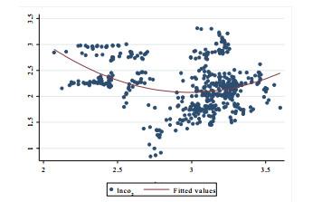
Prior to the panel data analysis, we plot tax burden against the CO

_{2}

emissions (Figure 1). As seen from Figure 1, carbon emissions per capita exhibited a negative trend with respect to tax burden at low levels. With an increasing tax burden, this relationship becomes positive. A more sophisticated analysis was therefore needed for exploring this relationship in depth.

Figure 1 Scatter plot: CO $_{2}$ emission per capita against the tax burden

Notes:

\ln {C O}_{2}

, lax denotes CO

_{2}

emission per capita and tax burden in natural logs, respectively.

Full size|PPT slide

4.2 Model Specification and Methodology

In order to clearly study the impact of tax burden on carbon dioxide emissions, based on the inclusion of tax burden in the STIRPAT model, combined with the actual situation and relevant literature, this chapter takes urbanization^[33] and trade openness^[34] as control variables into the model. This is mainly because urbanization is one of the important directions of modern economic and social reform. Rapid urbanization will lead to a sharp rise in energy demand. In particular, the contradiction between the rapid urbanization process and environmental protection is increasingly prominent. Therefore, it is particularly important to consider the impact of urbanization on carbon emissions. In addition, after the accession of OECD countries to the WTO, the scale of foreign trade has significantly improved. More and more frequent foreign trade will aggravate environmental problems. It is increasingly important to accurately determine the impact of pollution embodied in trade on the environment. Therefore, this chapter introduces the dependence degree of foreign trade into the econometric model. In conclusion, in order to study the impact of tax burden on carbon dioxide emissions in different quantiles, we have established the OECD national panel quantile regression measurement model, as follows:

\begin{array}{l} \ln {C O}_{2}_{i t} = α_{0} + β_{1} \ln {T a x}_{i t} + β_{2} \ln {T a x}_{i t}^{2} + β_{3} \ln {P G D P}_{i t} + β_{4} \ln {E C}_{i t} \\ + β_{5} \ln {P O P}_{i t} + β_{6} \ln {O p e n}_{i t} + β_{7} \ln {U r b a n}_{i t} + μ_{i} + ς_{t}, \end{array}

(4)

where CO

_{2}

are CO

_{2}

emission per capita,

T a x

denotes the tax burden measured by the ratio of tax revenue to GDP;

P G D P

is the gross product per capita;

E C

is the Energy use (kg of oil equivalent) per ＄1, 000 GDP (constant 2011 PPP);

P O P

denotes the population scale.

O p e n

represents the trade openness measured as the trade volume (% of GDP);

U r b a n

is the urban population (% of total).

μ_{i}

and

ς_{i}

are set to capture the individual and year fixed effects, respectively.

The effect of impact factors on CO

_{2}

emissions may be heterogeneity across the countries based on their level of CO

_{2}

emission^[32]. In order to investigate the heterogeneity of the effect of the tax burden at different levels of CO

_{2}

emissions, we employ a new panel quantile regression model with the non-additive fixed effects proposed by Powell^[35]. The main advantage of Powell's method relative to the existing quantile estimators with additive fixed effects (

α_{i})

is that it provides estimates of the distribution of

\ln {C O}_{2}_{i t}

given

D_{i t}

instead of

\ln {C O}_{2}_{i t} - α_{i}

given

D_{i t}

^[35]¹. The underlying model is

¹ Powell argues that the observations at the top of the (

\ln {C O}_{2}_{i t} - α_{i})

distribution may be at the bottom of the

\ln {C O}_{2}_{i t}

distribution and therefore additive fixed effect models cannot provide information about the effects of the policy variables on the outcome distribution^[35].

\ln {C O}_{2}_{i t} = \sum_{j = 1}^{7} D_{i t}^{'} β_{j} (U_{i t}^{*}),

(5)

where

\ln {C O}_{2}_{i t}

is the natural logarithms of CO

_{2}

emission for

i

country at

t

year;

β_{i t}

is the parameter of independent variables,

D_{i t}

is the set of explanatory variables, here, model contains seven explanatory variables: tax burden (

T a x)

and its quadratic term, per capita GDP (

P G D P)

, population scale (

P O P)

, urbanization (

U r b a n)

, per capita energy use (

E C)

, and trade openness (

O p e n)

U_{i t}^{*}

is the error term. The model is linear in parameters and

D_{i t}^{'} β (τ)

is strictly increasing in

τ

. For the

τ^{t h}

quantile of

\ln {C O}_{2}_{i t}

, quantile regression relies on the conditional restriction:

P (\ln {C O}_{2}_{i t} \leq D_{i t}^{'} β (τ) | D_{i t}) = τ .

(6)

Equation (6) indicates that the probability of the dependent variable is smaller than the quantile function is the same for all

D_{i t}

and equal to

τ

. Powell's QRPD estimator allows this probability to vary by individual and even within-individual as long as such variation is orthogonal to the instruments^[35]. Thus, QRPD relies on a conditional restriction and an unconditional restriction, letting

D_{i} = (D_{i t}, \dots, D_{i T}) :

\begin{array}{rcl} P (\ln {C O}_{2}_{i t} \leq D_{i t}^{'} β (τ) | D_{i t}) = P (\ln {C O}_{2}_{i t} \leq D_{i s}^{'} β (τ) | D_{i t}), \\ P (\ln {C O}_{2}_{i t} \leq D_{i t}^{'} β (τ)) = τ . \end{array}

(7)

Powell develops the estimator in an instrumental variables context given instruments

Z_{i t} = (Z_{i 1}, \dots, Z_{i T})

but notes that if the explanatory variables are exogenous (in which case

D_{i} = Z_{i})

many of the identification conditions are met trivially^[35]. The estimation uses the generalized method of moments (GMM). Sample moments are defined as:

\hat{g} (b) = \frac{1}{N} \sum_{i = 1}^{N} g_{i} (b)

with

\begin{array}{rcl} g_{i} (b) = \frac{1}{T} {\sum_{i = 1}^{T} (Z_{i t} - {\bar{Z}}_{i}) [1 (\ln {C O}_{2}_{i t} \leq D_{i t}^{'} b)]}, \end{array}

(8)

where

{\bar{Z}}_{i} = \frac{1}{T} \sum_{i = 1}^{T} Z_{i t}

Using Equation (8), the parameter set is defined as:

\begin{array}{rcl} B \equiv {b | τ - \frac{1}{N} \leq \frac{1}{N} \sum_{t = 1}^{N} 1 (\ln {C O}_{2}_{i t} \leq D_{i t}^{'} b) \leq τ}, \end{array}

(9)

for all

t

. Then, the parameter of interest is estimated as

\hat{β} (τ) = \arg min_{b \in β} {\hat{g}}^{'} (b) \hat{A} {\hat{g}}^{'} (b)

for some weighting matrix

\hat{A}

. The model is estimated by the Markov Chain Monte Carlo (MCMC) optimization method.

5 Empirical Findings

5.1 Panel Unit Root Test and Panel Cointegration Results

We check the stationary properties of variables by using the Fisher ADF unit root tests^[36], Fisher PP tests^[37] and LLC tests^[38]. Table 3 shows the results of the panel unit root test. It suggests that the variables are not stationary at the levels as the test statistics are unable to reject the null hypothesis of a panel unit root, albeit with the CO

_{2}

emission and energy use being an exception. However, all the variables are stationary at the first difference as the test statistics reject the null hypothesis of a panel unit root. Therefore, we conclude that these variables are integrated for order 1, I (1).

Table 3 Panel unit test

	Level			First difference
	LLC	ADF	PP	LLC	ADF	PP
$\ln {C O}_{2}$	$-$ 3.065***	54.471*	62.125**	$-$ 15.492***	280.814***	413.073***
	(0.001)	(0.094)	(0.023)	(0.000)	(0.000)	(0.000)
$\ln T a x$	0.829	17.445	17.064	$-$ 17.897***	337.251***	400.151***
	(0.796)	(1.000)	(1.000)	(0.000)	(0.000)	(0.000)
$\ln E C$	$-$ 10.221***	191.842***	264.265***	$-$ 13.250***	272.221***	326.586***
	(0.000)	(0.000)	(0.000)	(0.000)	(0.000)	(0.000)
$\ln P G D P$	10.930	1.259	0.566	$-$ 9.973***	170.349***	175.333***
	(1.000)	(1.000)	(1.000)	(0.000)	(0.000)	(0.000)
$\ln P O P$	4.821	16.179	34.455	$-$ 2.160**	57.599*	83.035***
	(1.000)	(1.000)	(0.789)	(0.015)	(0.055)	(0.000)
$\ln U r b a n$	$-$ 0.244	28.254	0.081	$-$ 9.134***	84.139***	110.833***
	(0.404)	(0.948)	(1.000)	(0.000)	(0.000)	(0.000)
$\ln O p e n$	4.964	4.8114	4.371	$-$ 19.181***	375.555***	387.514***
	(1.000)	(1.000)	(1.000)	(0.000)	(0.000)	(0.000)

Notes: *, **, *** are statistical significance at 10%, 5% and 1%, respectively. The significance probabilities for corresponding tests are reported in parentheses.

Unit root tests indicate that all the variables are integrated of order one, and then the panel cointegration test is applied to estimate whether there is a long-run equilibrium relationship among CO

_{2}

emission and these possible driving forces. We use three-panel cointegration tests: Pedroni^[39], Kao test^[40] and Fisher tests, and the results are presented in Table 4. According to Pedroni test, we find two out of the four panel-based statistics reveal evidence of panel cointegration among the variables at the 1% level of significance. Additionally, two of the three group test statistics reveal evidence of panel cointegration at a 1% level of significance. In sum, four of the seven tests suggest that there is panel cointegration among the variables in Equation (1). The Kao test also suggests panel cointegration at a 1% level of significance. In addition, the Johansen Fisher test suggests the existence of five cointegrating vectors at a 5% or better level of significance. Overall, there is strong statistical evidence in favour of panel cointegration among CO

_{2}

emissions, tax burden, per capita energy use, per capita GDP, urbanization and trade openness for the sample.

Table 4 Panel cointegration test

Panel 1 Pedroni test
Test statistics	Statistic	Prob.
Panel $v$ -Statistic (Weighted)	$-$ 2.635	0.996
Panel $ρ$ -Statistic (Weighted)	2.209	0.986
Panel PP-Statistic (Weighted)	$-$ 2.752***	0.003
Panel ADF-Statistic (Weighted)	$-$ 3.763***	0.000
Group $ρ$ -Statistic	4.143	1.000
Group PP-Statistic	$-$ 5.853***	0.000
Group ADF-Statistic	$-$ 6.293***	0.000
Panel 2 Fisher test
Hypothesized	Trace test	Max-eigen test
None	1135.000***	1441.000***
At most 1	804.600***	528.600***
At most 2	529.300***	394.900***
At most 3	315.500***	271.500***
At most 4	176.200***	195.000***
Panel 3 Kao test
	$t$ -Statistic	Prob.
ADF	$-$ 1.452*	0.073

Notes: *, **, *** are statistical significance at 10%, 5% and 1%, respectively. The null hypothesis is that there is no cointegration among variables. Lag length selection is based on SIC and is determined automatically with a max lag of 5.

5.2 Panel Causality Test

The finding of a panel long-run cointegration relationship among emissions, tax burden, per capita energy use, per capita GDP, urbanization and trade openness, suggests that there is Granger causality in at least one direction. This paper employs two approaches of causality testing in panels to examine the causal relationship between the CO

_{2}

emission and its impact factor. The first is to treat the panel data as one large stacked set of data, and then perform the Granger Causality test in the standard way, with the exception of not letting data from one cross-section enter the lagged values of data from the next cross-section. This method assumes that all coefficients are the same across all cross-sections. The second approach adopted by Dumitrescu and Hurlin, which allows all coefficients to be different across cross-sections^[41]. This paper mainly investigates the relationship between the tax burden and carbon emission. Therefore, we only list the test of causality between tax burden and per capita carbon emissions. The panel Granger causality results are presented in Table 5. By using the first approach, we find a un-bidirectional causality from tax burden to carbon emissions. Under the framework of Dumitrescu and Hurlin ^[41], we find that it rejects the null that

\ln T a x

does not homogeneously cause

\ln {C O}_{2}

. It reveals that the tax burden has a significant impact on carbon emission. Overall, there is strong statistical evidence in favour of causality running from tax burden to carbon emission, which deserves further study on how tax burden affects carbon emissions in the next section.

Table 5 Panel causality test

Panel causality test
Panel 1: Panel causality test: Stacked test
Null Hypothesis:	$F$ -Statistic
$\ln T a x$ does not Granger Cause $\ln {C O}_{2}$	3.042**
$\ln {C O}_{2}$ does not Granger Cause $\ln T a x$	0.945
Panel 2: Panel causality test: Pairwise Dumitrescu and Hurlin test^[41]
Null Hypothesis:	Zbar-Stat.
$\ln T a x$ does not homogeneously cause $\ln {C O}_{2}$	1.700*
$\ln {C O}_{2}$ does not homogeneously cause $\ln T a x$	$-$ 1.348

Notes: *, **, *** are statistical significance at 10%, 5% and 1%, respectively.

5.3 Panel Quantiles Results

To facilitate comparison, the model is estimated firstly by fixed effects OLS regression estimates. Columns (1), (2) and (3) in Table 6 present the pooled, one-way individual fixed effects and one-way time-period fixed-effects OLS regression estimates, respectively. These estimated results of three fixed-effect models show that after controlling the other variables, the coefficients for the tax burden and its quadratic term are not significant at the 10% significance levels. As pointed by Baltagi^[42], time-period fixed effects control for all time-specific, spatial-invariant variables whose omission could bias the estimates in a typical time series study. Thus, we focus our discussion on the results with respect to the model with a two-way fixed effect (see Equation (4)). To control such an effect, Column (4) reports the results of two-way fixed effects. The results still indicate that the tax burden has no impact on carbon emissions. Such results may be due to the fact that there panel regressions are based on conditional mean OLS estimation. We know OLS does not take into account the heterogeneity of the distribution, which may result in overestimation or underestimation^{[32, 43]}. Therefore, we turn to use a panel quantile model with fixed effect to further clarify the impact of the tax burden on carbon emissions.

Table 6 OLS regression results

	(1)	(2)	(3)	(4)
$\ln T a x$	$-$ 0.584	0.473	$-$ 0.084	0.238
	( $-$ 0.670)	(1.092)	( $-$ 0.100)	(0.565)
$\ln {T a x}^{2}$	0.049	$-$ 0.069	$-$ 0.044	$-$ 0.033
	(0.324)	( $-$ 0.939)	( $-$ 0.297)	( $-$ 0.467)
$\ln P G D P$	0.562***	0.891***	0.601***	0.902***
	(19.613)	(17.161)	(21.483)	(16.026)
$\ln E C$	0.392***	0.644***	0.306***	0.506***
	(7.785)	(15.725)	(6.170)	(12.794)
$\ln P O P$	0.066***	$-$ 0.520***	0.097***	0.010
	(4.161)	( $-$ 5.678)	(6.099)	(0.097)
$\ln U r b a n$	0.040	0.310*	0.371***	1.108***
	(0.338)	(1.741)	(3.083)	(6.103)
$\ln O p e n$	0.202***	$-$ 0.310***	0.326***	$-$ 0.193***
	(5.004)	( $-$ 9.402)	(7.678)	( $-$ 5.372)
$C$	$-$ 6.400***	$-$ 2.530*	$-$ 9.516***	$-$ 14.276***
	( $-$ 4.022)	( $-$ 1.589)	( $-$ 6.040)	( $-$ 7.296)
Province	-	yes	-	yes
Year	-	-	yes	yes
$R^{2}$	0.548	0.966	0.604	0.974

Notes: *, **, *** are statistical significance at 10%, 5% and 1%, respectively.

In order to control the distributional heterogeneity and further investigate whether the impact of the tax burden on CO

_{2}

emissions is varying across the countries based on their level of CO

_{2}

emission, a panel quantile regression with the non-additive fixed effects proposed by Powell is used in this paper^[35]. Quantile regression is able to describe the entire conditional distribution of the dependent variable (CO

_{2}

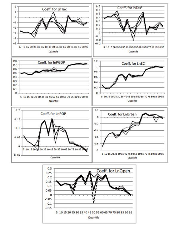
emissions). Using this model, we are able to assess the determinants of carbon emissions throughout the conditional distribution, with a particular focus on the most and least emissions countries. To see the dynamics of estimated elasticity for the effect of key factors on carbon emissions across different quantiles, this paper lists the curve of coefficient in Figure 2. The results are reported for the 10

^{t h}

, 20

^{t h}

, 30

^{t h}

, 40

^{t h}

, 50

^{t h}

, 60

^{t h}

, 70

^{t h}

, 80

^{t h}

, 90

^{t h}

percentiles of the conditional emissions distribution in Table 3. The empirical results show that the impacts of various factors, particularly the tax burden, on carbon emissions are heterogeneous.

Figure 2 Dynamic of panel quantile regressions coefficients

Notes: The dashed line represents the 95% confidence interval for the quantile regression estimator.

Full size|PPT slide

Regarding tax burden, as seen in Table 3 and Figure 2, at different quantiles, the coefficients of the tax burden (

\ln T a x)

with respect to CO

_{2}

emissions are clear heterogeneous, but supporting evidence that an increase in tax burden is associated with a decrease in CO

_{2}

emissions as a whole. More specifically, it shows that at the lower quantiles such as 10

^{t h}

, 20

^{t h}

and 40

^{t h}

quantiles, which responding to the lower CO

_{2}

emission countries, the coefficient of

\ln T a x

-

2.889,

-

3.2 and

-

2.070, and significantly at the 10% level. In contrast, at the higher quantile such as 80

^{t h}

and 90

^{t h}

quantiles, which responding to the higher CO

_{2}

emission countries, the coefficient of

\ln T a x

-

0.716 and

-

1.483, and passes the significant test at the 10% level, respectively. By comparing the size of the coefficient of

\ln T a x

in the lower quantiles and higher quantiles, it reveals that the increase of tax burden has a much greater effect on reducing the carbon emissions in these countries with fewer carbon emissions than in those countries with higher carbon emissions. We also use a quadratic term of the tax burden to capture a possible non-linear relationship between carbon emissions and tax burden. The results indicate that the coefficients of the squared tax burden (

\ln {T a x}^{2})

are positive and significant, indicating there exists a U-shaped relationship between tax burden and CO

_{2}

emissions in the O

E C

D countries. It means that there is one threshold value for tax burden in sampled countries with different levels of carbon emissions. CO

_{2}

emissions first decrease with an increase in tax burden and then the growth of tax burden increases the CO

_{2}

emissions when the tax burden is above the threshold value.

For control variables, as can be seen from Table 7 and Figure 2, at each quantile, the coefficients of per capita GDP and energy use are positive and significant at 10% significance level. It reveals the GDP and energy intensity has positive impacts on the carbon emission for each economy at a different level of CO

_{2}

emissions. This finding is consistent with existing literature such as Menz and Welsch who report that an increase in economic growth and energy consumption is associated with an increase in emissions based on the data of 26 O

E C

D countries^[44]. However, unlike most studies, this paper further provides evidence that there exists a heterogeneous effect of them on the carbon emission across different quantiles. As seen in Figure 2, with the quantiles increasing, i.e., with CO

_{2}

emissions increasing, the size of the effect of the per capita GDP and energy intensity on CO

_{2}

emission increases. That is, the size of the effect of per capita GDP and energy intensity on CO

_{2}

emissions at the lower quantiles is smaller than that at the higher quantiles. It indicates that the increase in the GDP and energy intensity has a much greater effect on increasing carbon emissions in O

E C

D countries with higher carbon emissions than in those countries with lower carbon emissions.

Table 7 Quantile regression results

	0.1	0.2	0.3	0.4	0.5	0.6	0.7	0.8	0.9
$\ln T a x$	$-$ 2.889***	$-$ 3.200***	$-$ 1.516***	$-$ 2.070***	0.035	$-$ 1.991***	0.185***	$-$ 0.716***	$-$ 1.483***
	( $-$ 1712.67)	( $-$ 611.87)	( $-$ 7.080)	( $-$ 13.730)	(0.07)	( $-$ 6.32)	(2.32)	( $-$ 16.76)	( $-$ 21.18)
$\ln {T a x}^{2}$	0.423***	0.482***	0.246***	0.308***	$-$ 0.034	0.342***	0.030***	0.124***	0.255***
	(1369.07)	(529.11)	(6.69)	(10.28)	( $-$ 0.39)	(6.39)	(2.13)	(15.77)	(21.59)
$\ln P G D P$	0.507***	0.457***	0.509***	0.552***	0.582***	0.558***	0.684***	0.720***	0.716***
	(11000)	(8379)	(87.93)	(39.59)	(23.84)	(85.53)	(270.3)	(178.52)	(479.04)
$\ln E C$	0.163***	0.268***	0.646***	0.507***	0.611***	0.647***	0.871***	0.952***	0.970***
	(852.03)	(829.88)	(87.37)	(18.68)	(28.06)	(71.62)	(136.62)	(110.1	488.08
$\ln P O P$	0.029***	0.002***	0.120***	0.067***	0.062***	0.094***	0.019***	0.006***	$-$ 0.012***
	(1771.01)	(21.41)	(49.97)	(16.1)	(2.64)	(17.26)	(9.78)	(3.84)	( $-$ 11.82)
$\ln U r b a n$	$-$ 0.633***	$-$ 0.472***	$-$ 0.546***	$-$ 0.436***	$-$ 0.213***	$-$ 0.208***	0.111***	0.063***	0.016***
	( $-$ 5228.85)	( $-$ 1902.64)	$-$ 56.06	( $-$ 8.00)	( $-$ 5.070)	( $-$ 10.840)	(17.58)	(8.43)	(3.48)
$\ln O p e n$	0.105***	0.118***	0.180***	0.134***	0.052	0.178***	0.094***	0.071***	0.036***
	(1924.5)	(441.71)	(35.94)	(14.65)	(0.7)	(18.87)	(24.1)	(9.56)	(14.28)

Notes: *, **, *** are statistical significance at 10%, 5% and 1%, respectively.

Concerning population factors, it shows that the population size has a positive impact on the carbon emissions at most quantiles. It indicates that the increase in population-scale will lead to an increase in carbon emissions. This finding is in line with Shafiei and Salim who obtain the same results for O

E C

D countries^[45]. By contrast, it shows that urbanization has a heterogeneous effect on carbon emission across different quantiles. In particular, at the lower quantiles such as 10

^{t h}

, 20

^{t h}

, 30

^{t h}

and 40

^{t h}

, the coefficients of urbanization with respect to carbon emission are negative and significant at 10% significances levels. It means that the increases in urbanization are associated with the decreases in carbon emissions for these countries with lower carbon emissions. However, at the higher quantiles such as 70

^{t h}

, 80

^{t h}

and 90

^{t h}

, which responding to the higher CO

_{2}

emission countries, the coefficients of urbanization are 0.111, 0.063 and 0.016, and pass the significant test at the 10% level respectively as well. It reveals that for countries with higher carbon emissions, the expansion of urbanization will lead to an increase in carbon emissions.

With regard to trade openness, Figure 2 shows that the coefficients of trade openness are positive and significant at each quantile. It indicates the trade openness positively affect the carbon emission. The finding is in line with Sharma who provides evidence support that the increases in the trade openness are associated with the increases of carbon emissions based on 69 countries data over the period from 1985 to 2005^[46].

5.4 Robustness Analysis

5.4.1 Estimation based on new quantiles

According to Subsection 5.3, we know, the lower quantiles (e.g., 10

^{t h}

, 20

^{t h}

, 30

^{t h})

responding to the lower CO

_{2}

emission countries, and higher quantiles (e.g., 70

^{t h}

, 80

^{t h}

, 90

^{t h})

responding to the higher CO

_{2}

emission countries. However, the estimated parameters may be insignificant at these special quantiles we set. To test the robustness of the results and examine whether this setting of quantiles will lead to the changes of our results, we reset 9 quantiles, i.e., 5

^{t h}

, 15

^{t h}

, 25

^{t h}

, 35

^{t h}

, 45

^{t h}

, 55

^{t h}

, 65

^{t h}

, 75

^{t h}

, 85

^{t h}

percentiles. The results for these new percentiles of the conditional emissions distribution are reported in Table 8. We still find that at different quantiles, there is a U-shaped relationship between the tax burden and carbon emissions. Our results are robust.

Table 8 Panel quantile regression with the new setting of percentiles

	0.05	0.15	0.25	0.35	0.45	0.55	0.65	0.75	0.85
$\ln T a x$	$-$ 2.647***	$-$ 2.854***	$-$ 3.200***	$-$ 0.349***	$-$ 0.615***	$-$ 1.2658***	$-$ 2.897***	$-$ 0.806***	$-$ 0.762***
	( $-$ 270.860)	( $-$ 1529.29)	( $-$ 9.280)	( $-$ 3.440)	( $-$ 10.230)	( $-$ 9.08)	( $-$ 21.11)	( $-$ 18.47)	( $-$ 3.33)
$\ln {T a x}^{2}$	0.370***	0.415***	0.469***	0.053***	0.102***	0.198***	0.502***	0.142***	0.139***
	(222.23)	(1302.53)	(8.62)	(3.15)	(9.47)	(9.1)	(21.04)	(20.76)	(3.57)
$\ln P G D P$	0.485***	0.457***	0.535***	0.561***	0.558***	0.554***	0.561***	0.705***	0.728***
	(2218.48)	(4003.04)	(62.79)	(119.8)	(116.05)	(124.57)	(163.38)	(470.87)	(119.24)
$\ln E C$	0.295	0.149***	0.402***	0.692***	0.713***	0.629***	0.643***	0.915***	0.994***
	(0.295)	(729.87)	(14.41)	(90.48)	(130.25)	(56.07)	(145.35)	(410.52)	(79.09)
$\ln P O P$	0.058***	0.016***	0.003	0.142***	0.151***	0.102***	0.080***	0.019***	0.002
	(671.29)	(144.75)	(0.23)	(122.23)	(61.32)	(25.33)	(45.16)	(7.48)	(0.77)
$\ln U r b a n$	$-$ 0.888***	$-$ 0.508***	$-$ 0.579***	$-$ 0.402***	$-$ 0.363***	$-$ 0.207***	0.066***	0.043***	$-$ 0.037***
	( $-$ 945.240)	( $-$ 2638.60)	$-$ 17.81	$-$ 36.22	$-$ 18.47	( $-$ 11.390)	(9.47)	(5.2)	( $-$ 0.600)
$\ln O p e n$	0.157***	0.126***	0.060***	0.219***	0.264***	0.213***	0.222***	0.073***	0.075***
	(788.2)	(512.92)	(2.32)	(36.95)	(57.98)	(15.53)	(53.22)	(54.34)	(5.62)

Notes:

Z

statistic in the parentheses.
*, **, *** are statistical significance at 10%, 5% and 1%, respectively.

5.4.2 Evidence from G7 countries

As the earliest countries to start the industrialized revolution, the G7 countries are an important part of O

E C

D. Their rich and vast experience in tackling environmental challenges provides a reference for the design of energy saving and pollution reduction policies in developing countries. Therefore, we examine whether our main inclusions are valid in G7 countries. Table 9 shows the regression results. Under the framework of the panel quantiles model, we still find a U-shaped relationship between the tax burden and carbon emissions for G7 countries.

Table 9 Quantile regression results for G7 countries

	0.1	0.2	0.3	0.4	0.5	0.6	0.7	0.8	0.9
$\ln T a x$	$-$ 1.996**	$-$ 1.397***	1.594	$-$ 1.308*	$-$ 2.501***	$-$ 2.258***	$-$ 1.525*	$-$ 0.0195	$-$ 0.254***
	( $-$ 2.83)	( $-$ 3.31)	$-$ 1.13	( $-$ 2.26)	( $-$ 3.85)	( $-$ 10.82)	( $-$ 1.95)	( $-$ 0.05)	( $-$ 3.79)
$\ln {T a x}^{2}$	0.266*	0.162*	$-$ 0.251	0.260*	0.476***	0.434***	0.293*	0.017	0.054***
	(2.06)	(2.37)	( $-$ 1.03)	(2.55)	(4.11)	(12.29)	(2.18)	(0.25)	(4.5)
$\ln P G D P$	1.478***	1.015***	0.732***	0.800***	0.830***	0.852***	0.837***	0.880***	0.705***
	(11.96)	(4.57)	(5.88)	(17.84)	(38.05)	(11.3)	(4.89)	(29.6)	(108.54)
$\ln E C$	1.208***	1.165***	1.108***	1.018***	1.028***	1.058***	0.994***	0.911***	0.894***
	(50.93)	(16.44)	(28.87)	(29.29)	(184.15)	(104.2)	(25.99)	(96.9)	(185.05)
$\ln P o p u$	0.128**	0.182	0.371**	0.224***	0.220***	0.203***	0.177***	0.164***	0.142***
	(3.25)	(1.45)	(3.05)	(8.54)	(10.45)	(20.67)	(8.96)	(14.24)	(66.82)
$\ln U r b a n$	$-$ 3.192***	$-$ 2.282***	$-$ 1.208*	$-$ 0.877***	$-$ 1.093***	$-$ 1.144***	$-$ 1.421***	$-$ 0.902***	$-$ 0.634***
	( $-$ 29.70)	( $-$ 14.55)	( $-$ 2.43)	( $-$ 10.27)	( $-$ 12.15)	( $-$ 9.94)	( $-$ 3.39)	( $-$ 21.71)	( $-$ 30.06)
$\ln O p e n$	0.105**	0.169	0.317*	0.135***	0.163***	0.131***	0.0582***	$-$ 0.016	$-$ 0.024***
	(2.63)	(1.05)	(2.22)	(6.19)	(6.87)	(6.18)	(3.35)	( $-$ 1.59)	( $-$ 4.30)
$N$	168	168	168	168	168	168	168	168	168

Notes:

Z

statistic in the parentheses.
*, **, *** are statistical significance at 10%, 5% and 1%, respectively.

6 Conclusion

In this paper, we have investigated the relationship between tax burden and carbon emissions using data from a cross-section of O

E C

D countries over the time span from 1991 to 2014. To examine whether the impact of the tax burden on carbon emissions varies across the countries based on their levels of carbon emissions, we have employed a new panel quantile model with fixed effect to investigate the impact of the tax burden on environmental quality. The main conclusions can be drawn as follows:

Firstly, we find (ⅰ) the impact of the tax burden on carbon emissions is heterogeneous across countries based on the level of carbon emissions, but (ⅱ) it always in favour of U-shaped relationship between the tax burden and carbon emissions for countries with different levels of carbon emission. It means that when the tax burden exceeds a threshold value, the relationship between tax burden and carbon emissions will turn from negative to positive. This finding suggests that moderate taxes could help reduce carbon emissions, but excessive taxation has the opposite impact.

Secondly, there exist heterogeneous effects of control variables on the carbon emissions across different quantiles as well. More specifically, we find that (ⅰ) the increase of the GDP and energy intensity have a much greater effect on increasing carbon emissions in O

E C

D countries with higher carbon emissions than in those countries with lower carbon emissions. (ⅱ) Whether in high-carbon or low-carbon countries, we find that population size and trade openness has a positive impact on carbon emissions, respectively. (ⅲ) Increasing urbanization can decrease the carbon emissions in countries with smaller carbon emissions, while it has a positive impact on carbon emissions in higher carbon emissions countries.

Based on these findings, we propose some policy implications. Firstly, we find that there is a U-shaped relationship between the tax burden and carbon emissions, which indicates that excessive taxation is not conducive to reducing carbon emissions. Enterprises and individuals are important participants in the process of carbon reduction. Therefore, governments should pay more attention to the impact of the tax burden on enterprises and individuals when they are actively discharging their carbon responsibilities. Our finding suggests that the government should control the level of the tax burden and keep it within a reasonable scope, so as to avoid the harm caused by the excessive tax burden to enterprises and individuals.

Secondly, governments around the world should adjust their tax policy rationally according to the state of economic growth. If the current economy is recessionary or slowly developing, governments should lower taxes or increase fiscal spending to compensate companies that are actively reducing emissions, thereby reducing the negative impact of tax burdens on businesses. For example, the government can offer financial incentives or tax care to companies that proactively reduce emissions by means of technological innovation.

Thirdly, governments should rationally optimize their fiscal expenditure and ensure that the investment in environmental governance is stable. When the governments adjust their tax policy, especially the tax cuts will reduce their revenue, which may affect the government's investment in environmental governance. Therefore, if governments are prepared to cut taxes, they should take other policies such as a modest increase in government deficits to ensure a steady increase in the investment in environmental governance.

It is noteworthy that there are still many relevant studies that merit future efforts: For example, it can further examine whether the impacts of the tax burden in the individual and corporate on carbon emissions are different. In addition, our conclusion is based on data from developed O

E C

D countries. In the future, it can further study the relationship between tax burdens and carbon emissions in developing countries, meanwhile, estimate whether there are differences between the developed countries and developing countries.

References

Publishing order | Descend order by publishing year | Descend order by cited within

1	Kuo T C, Hong I H, Lin S C. Do carbon taxes work? Analysis of government policies and enterprise strategies in equilibrium. Journal of Cleaner Production, 2016, 139, 337- 346. https://doi.org/10.1016/j.jclepro.2016.07.164 Cited in this article [1]

2	Frey M. Assessing the impact of a carbon tax in Ukraine. Climate Policy, 2017, 17(3): 378- 396. https://doi.org/10.1080/14693062.2015.1096230 Cited in this article [1]

3	Lin B, Li X. The effect of carbon tax on per capita CO₂ emissions. Energy Policy, 2011, 39(9): 5137- 5146. https://doi.org/10.1016/j.enpol.2011.05.050 Cited in this article [3]

4	Meng S, Siriwardana M, McNeill J. The environmental and economic impact of the carbon tax in Australia. Environmental and Resource Economics, 2013, 54(3): 313- 332. https://doi.org/10.1007/s10640-012-9600-4 Cited in this article [1]

5	Benavente J M G. Impact of a carbon tax on the Chilean economy: A computable general equilibrium analysis. Energy Economics, 2016, 57, 106- 127. https://doi.org/10.1016/j.eneco.2016.04.014 Cited in this article [1]

6	Kneller R, Bleaney M F, Gemmell N. Fiscal policy and growth: Evidence from OECD countries. Journal of Public Economics, 1999, 74(2): 171- 190. https://doi.org/10.1016/S0047-2727(99)00022-5 Cited in this article [1]

7	Padovano F, Galli E. Tax rates and economic growth in the OECD countries. Economic Inquiry, 2001, 39(1): 44- 57. https://doi.org/10.1093/ei/39.1.44 Cited in this article [1]

Greening L A, Ting M, Krackler T J. Effects of changes in residential end-uses and behavior on aggregate carbon intensity: Comparison of 10 OECD countries for the period 1970 through 1993. Energy Economics, 2001, 23(2): 153- 178.

https://doi.org/10.1016/S0140-9883(00)00059-1

Cited in this article [1]

9	Hall B, Van Reenen J. How effective are fiscal incentives for R&D? A review of the evidence. Research Policy, 2000, 29(4-5): 449- 469. https://doi.org/10.1016/S0048-7333(99)00085-2 Cited in this article [1]

10	Czarnitzki D, Hanel P, Rosa J M. Evaluating the impact of R&D tax credits on innovation: A microeconometric study on Canadian firms. Research Policy, 2011, 40(2): 217- 229. https://doi.org/10.1016/j.respol.2010.09.017 Cited in this article [1]

11	Noailly J. Improving the energy efficiency of buildings: The impact of environmental policy on technological innovation. Energy Economics, 2012, 34(3): 795- 806. https://doi.org/10.1016/j.eneco.2011.07.015 Cited in this article [1]

12	Costa-Campi M T, García-Quevedo J, Segarra A. Energy efficiency determinants: An empirical analysis of Spanish innovative firms. Energy Policy, 2015, 83, 229- 239. https://doi.org/10.1016/j.enpol.2015.01.037 Cited in this article [1]

13	Bruvoll A, Larsen B M. Greenhouse gas emissions in Norway: do carbon taxes work?. Energy Policy, 2004, 32(4): 493- 505. https://doi.org/10.1016/S0301-4215(03)00151-4 Cited in this article [1]

14	Lu C, Tong Q, Liu X. The impacts of carbon tax and complementary policies on Chinese economy. Energy Policy, 2010, 38(11): 7278- 7285. https://doi.org/10.1016/j.enpol.2010.07.055 Cited in this article [1]

15	Guo Z, Zhang X, Zheng Y, et al. Exploring the impacts of a carbon tax on the Chinese economy using a CGE model with a detailed disaggregation of energy sectors. Energy Economics, 2014, 45, 455- 462. https://doi.org/10.1016/j.eneco.2014.08.016 Cited in this article [1]

16	Liu L, Huang C Z, Huang G, et al. How a carbon tax will affect an emission-intensive economy: A case study of the Province of Saskatchewan, Canada. Energy, 2018, 159, 817- 826. https://doi.org/10.1016/j.energy.2018.06.163 Cited in this article [1]

17	Loganathan N, Shahbaz M, Taha R. The link between green taxation and economic growth on CO₂ emissions: Fresh evidence from Malaysia. Renewable and Sustainable Energy Reviews, 2014, 38, 1083- 1091. https://doi.org/10.1016/j.rser.2014.07.057 Cited in this article [1]

18	Lopez R E, Palacios A. Have government spending and energy tax policies contributed to make Europe environmentally cleaner? University of Maryland, Maryland, Working Paper 94795, 2010. Cited in this article [1]

19	López R, Galinato G I, Islam A. Fiscal spending and the environment: Theory and empirics. Journal of Environmental Economics and Management, 2011, 62(2): 180- 198. https://doi.org/10.1016/j.jeem.2011.03.001 Cited in this article [2]

20	Halkos G E, Paizanos E A. The effect of government expenditure on the environment: An empirical investigation. Ecological Economics, 2013, 91, 48- 56. https://doi.org/10.1016/j.ecolecon.2013.04.002 Cited in this article [1]

21	López R, Palacios A. Why has Europe become environmentally cleaner? Decomposing the roles of fiscal, trade and environmental policies. Environmental and Resource Economics, 2014, 58(1): 91- 108. https://doi.org/10.1007/s10640-013-9692-5 Cited in this article [1]

22	Islam, A M, López, R E. Government spending and air pollution in the US. International Review of Environmental and Resource Economics, 2015, 8(2): 139- 189. https://doi.org/10.1561/101.00000068 Cited in this article [1]

23	Galinato G I, Galinato S P. The effects of government spending on deforestation due to agricultural land expansion and CO₂ related emissions. Ecological Economics, 2016, 122, 43- 53. https://doi.org/10.1016/j.ecolecon.2015.10.025 Cited in this article [1]

24	Halkos G E, Paizanos E A. The effects of fiscal policy on CO₂ emissions: Evidence from the USA. Energy Policy, 2016, 88, 317- 328. https://doi.org/10.1016/j.enpol.2015.10.035 Cited in this article [1]

25	Zhang Q, Zhang S, Ding Z, et al. Does government expenditure affect environmental quality? Empirical evidence using Chinese city-level data. Journal of Cleaner Production, 2017, 161, 143- 152. https://doi.org/10.1016/j.jclepro.2017.05.096 Cited in this article [1]

26	Ehrlich P R, Holdren J P. Impact of population growth. Science, 1971, 171(3977): 1212- 1217. https://doi.org/10.1126/science.171.3977.1212 Cited in this article [1]

27	Dietz T, Rosa E A. Effects of population and affluence on CO₂ emissions. Proceedings of the National Academy of Sciences, 1997, 94(1): 175- 179. https://doi.org/10.1073/pnas.94.1.175 Cited in this article [1]

28	Martínez-Zarzoso I, Maruotti A. The impact of urbanization on CO₂ emissions: Evidence from developing countries. Ecological Economics, 2011, 70(7): 1344- 1353. https://doi.org/10.1016/j.ecolecon.2011.02.009 Cited in this article [1]

29	Adewuyi A O. Effects of public and private expenditures on environmental pollution: A dynamic heterogeneous panel data analysis. Renewable and Sustainable Energy Reviews, 2016, 65, 489- 506. https://doi.org/10.1016/j.rser.2016.06.090 Cited in this article [1]

30	Ma C, Rogers A A, Kragt M E, et al. Consumers' willingness to pay for renewable energy: A metaregression analysis. Resource and Energy Economics, 2015, 42, 93- 109. https://doi.org/10.1016/j.reseneeco.2015.07.003 Cited in this article [1]

31	Vegh C A, Vuletin G. How is tax policy conducted over the business cycle?. American Economic Journal: Economic Policy, 2015, 7(3): 327- 370. https://doi.org/10.1257/pol.20120218 Cited in this article [1]

32	Zhu H, Duan L, Guo Y, et al. The effects of FDI, economic growth and energy consumption on carbon emissions in ASEAN-5:Evidence from panel quantile regression. Economic Modelling, 2016, 58, 237- 248. https://doi.org/10.1016/j.econmod.2016.05.003 Cited in this article [3]

33	Xu B, Lin B. Factors affecting CO₂ emissions in China's agriculture sector: Evidence from geographically weighted regression model. Energy Policy, 2017, 104, 404- 414. https://doi.org/10.1016/j.enpol.2017.02.011 Cited in this article [1]

34	Shahbaz M, Nasreen S, Ahmed K, et al. Trade openness-carbon emissions nexus: The importance of turning points of trade openness for country panels. Energy Economics, 2017, 61, 221- 232. https://doi.org/10.1016/j.eneco.2016.11.008 Cited in this article [1]

35	Powell D. Quantile regression with nonadditive fixed effects. Quantile Treatment Effects, 2016, 1- 28. Cited in this article [6]

36	Maddala G S, Wu S. A comparative study of unit root tests with panel data and a new simple test. Oxford Bulletin of Economics and Statistics, 1999, 61(S1): 631- 652. https://doi.org/10.1111/1468-0084.0610s1631 Cited in this article [1]

37	Choi I. Unit root tests for panel data. Journal of international money and Finance, 2001, 20(2): 249- 272. https://doi.org/10.1016/S0261-5606(00)00048-6 Cited in this article [1]

38	Levin A, Lin C F, Chu C S J. Unit root tests in panel data: Asymptotic and finite-sample properties. Journal of Econometrics, 2002, 108(1): 1- 24. https://doi.org/10.1016/S0304-4076(01)00098-7 Cited in this article [1]

39	Pedroni P. Panel cointegration: Asymptotic and finite sample properties of pooled time series tests with an application to the PPP hypothesis. Econometric Theory, 2004, 20(3): 597- 625. Cited in this article [1]

40	Kao C. Spurious regression and residual-based tests for cointegration in panel data. Journal of Econometrics, 1999, 90(1): 1- 44. https://doi.org/10.1016/S0304-4076(98)00023-2 Cited in this article [1]

41	Dumitrescu E I, Hurlin C. Testing for Granger non-causality in heterogeneous panels. Economic Modelling, 2012, 29(4): 1450- 1460. https://doi.org/10.1016/j.econmod.2012.02.014 Cited in this article [3]

42	Baltagi B. Econometric analysis of panel data. John Wiley & Sons, 2008. Cited in this article [1]

43	Hübler M. The inequality-emissions nexus in the context of trade and development: A quantile regression approach. Ecological Economics, 2017, 134, 174- 185. https://doi.org/10.1016/j.ecolecon.2016.12.015 Cited in this article [1]

44	Menz T, Welsch H. Population aging and carbon emissions in OECD countries: Accounting for life-cycle and cohort effects. Energy Economics, 2012, 34(3): 842- 849. https://doi.org/10.1016/j.eneco.2011.07.016 Cited in this article [1]

45	Shafiei S, Salim R A. Non-renewable and renewable energy consumption and CO₂ emissions in OECD countries: A comparative analysis. Energy Policy, 2014, 66, 547- 556. https://doi.org/10.1016/j.enpol.2013.10.064 Cited in this article [1]

46	Sharma S S. Determinants of carbon dioxide emissions: Empirical evidence from 69 countries. Applied Energy, 2011, 88(1): 376- 382. https://doi.org/10.1016/j.apenergy.2010.07.022 Cited in this article [1]

PDF(470 KB)

249

Accesses

Citation

Detail

Sections

Recommended

Abstract
Key words
Cite this article
1 Introduction
2 Literature
2.1 Carbon Tax and Carbon Emission
2.2 Fiscal Policy (Tax) and Environment
3 Theoretical Framework and Hypothesis
4 Data, Model Specification, and Methodology
4.1 Data
Table 1 Basic information about the variables
Table 2 Descriptive statistics
Figure 1 Scatter plot: CO $_{2}$ emission per capita against the tax burden
4.2 Model Specification and Methodology
5 Empirical Findings
5.1 Panel Unit Root Test and Panel Cointegration Results
Table 3 Panel unit test
Table 4 Panel cointegration test
5.2 Panel Causality Test
Table 5 Panel causality test
5.3 Panel Quantiles Results
Table 6 OLS regression results
Figure 2 Dynamic of panel quantile regressions coefficients
Table 7 Quantile regression results
5.4 Robustness Analysis
5.4.1 Estimation based on new quantiles
Table 8 Panel quantile regression with the new setting of percentiles
5.4.2 Evidence from G7 countries
Table 9 Quantile regression results for G7 countries
6 Conclusion
References

Received	Accepted	Published
2020-03-14	2020-05-14	2021-08-25
Issue Date
2021-08-25

Please choose a citation manager

Content to export

Abstract

Key words

Cite this article

1 Introduction

2 Literature

2.1 Carbon Tax and Carbon Emission

2.2 Fiscal Policy (Tax) and Environment

3 Theoretical Framework and Hypothesis

4 Data, Model Specification, and Methodology

4.1 Data

Table 1 Basic information about the variables

Table 2 Descriptive statistics

Figure 1 Scatter plot: CO $_{2}$ emission per capita against the tax burden

4.2 Model Specification and Methodology

5 Empirical Findings

5.1 Panel Unit Root Test and Panel Cointegration Results

Table 3 Panel unit test

Table 4 Panel cointegration test

5.2 Panel Causality Test

Table 5 Panel causality test

5.3 Panel Quantiles Results

Table 6 OLS regression results

Figure 2 Dynamic of panel quantile regressions coefficients

Table 7 Quantile regression results

5.4 Robustness Analysis

5.4.1 Estimation based on new quantiles

Table 8 Panel quantile regression with the new setting of percentiles

5.4.2 Evidence from G7 countries

Table 9 Quantile regression results for G7 countries

6 Conclusion

{{custom_sec.title}}

{{custom_sec.title}}

References

{{custom_fnGroup.title_en}}

Footnotes

Share

模态框（Modal）标题

Please choose a citation manager

Content to export

Abstract

Key words

Cite this article

1 Introduction

2 Literature

2.1 Carbon Tax and Carbon Emission

2.2 Fiscal Policy (Tax) and Environment

3 Theoretical Framework and Hypothesis

4 Data, Model Specification, and Methodology

4.1 Data

Table 1 Basic information about the variables

Table 2 Descriptive statistics

Figure 1 Scatter plot: CO2 emission per capita against the tax burden

4.2 Model Specification and Methodology

5 Empirical Findings

5.1 Panel Unit Root Test and Panel Cointegration Results

Table 3 Panel unit test

Table 4 Panel cointegration test

5.2 Panel Causality Test

Table 5 Panel causality test

5.3 Panel Quantiles Results

Table 6 OLS regression results

Figure 2 Dynamic of panel quantile regressions coefficients

Table 7 Quantile regression results

5.4 Robustness Analysis

5.4.1 Estimation based on new quantiles

Table 8 Panel quantile regression with the new setting of percentiles

5.4.2 Evidence from G7 countries

Table 9 Quantile regression results for G7 countries

6 Conclusion

{{custom_sec.title}}

{{custom_sec.title}}

References

{{custom_fnGroup.title_en}}

Footnotes

Figure 1 Scatter plot: CO $_{2}$ emission per capita against the tax burden