1 Introduction
There are non-linear and volatile characters of the foreign exchange rate data, and it is not efficient to forecast by current statistical models
[1]. Financial time series forecasting is one of the most challenging problems, and artificial neural networks (ANNs) are used to solve this problem. The performance of the time series forecasting model, however, is limited by its low accuracy for forecasting longer periods. In this paper, the wavelet-based Elman neural network, which was applied with the modified differential evolution algorithm integratedly, is proposed to forecast foreign exchange rates.
ANNs performs better than the traditional statistical models such as ARIMA in forecasting the foreign exchange rate. Kadilar, et al.
[2] explored both the ARIMA model and neural networks for the Turkish TL/US dollar exchange rate series. Results show that the ANN method has far better accuracy compared to the ARIMA time series model. Naeini, et al.
[3] compared the feedforward multilayer perceptron (MLP) with a modified Elman neural network (ENN) model to predict a company stock value. The results show that the modified ENN has lower MSE, MAPE, and MAE values in comparison with MLP. ENN has dynamic characteristics, which are provided by internal connections. To the structure of ENN, it does not require the state as an input or training signal. This makes it superior to static feedforward networks, and can be widely used in a dynamic system
[4-6]. The performance of ENN is greatly affected by parameters. PSO, GA, and other optimal algorithms are applied to train the parameters of ENN
[7-12]. According to the researches of Ciarlini
[13], Lei
[14], Ong
[15], et al., the transfer function of the hidden layer is another important factor that affects the forecasting accuracy of ENN. Zhang and Benveniste
[16] applied the wavelet function to the hidden layer of the BP neural network and proposed the wavelet neural network (WNN). The performance of WNN improved a lot by doing this. Zhang
[17] studied the frames of wavelet.
In this work, we firstly apply wavelet function to the hidden layer of ENN, and we expect the performance of it would improve as WNN. Lu, et al.
[18] proposed a recurrent wavelet-based Elman neural network, which was used to control hybrid offshore wind and wave power generation systems, and derived optimal learning rates to adjust the network parameters. Then, we use an improved differential evolution (DE) algorithm to train the parameters of ENN. DE, first reported by Storn and Price
[19], is easy to implement, has few parameters to control, and can improve the performance through just changing parameters without imposing computation burden
[20-24]. The DE family of algorithms has been frequently adopted to tackle multi-objective, constrained, dynamic, large-scale, and multimodal optimization problems
[25-29]. The simulation was made to find how did the wavelet function and the modified DE algorithm improve the performance of ENN.
2 Elman Neural Network with Wavelet Transfer Function
2.1 Elman Neural Network
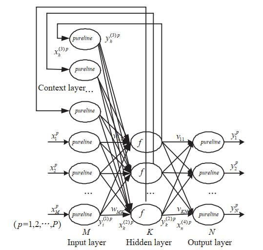
ENN originally developed by Elman in 1990 based on the Jordan network
[30]. The structure of ENN contains four parts
[31, 32]: The input layer, hidden layer, context layer and output layer, which is illustrated in
Figure 1. Considering the structure of ENN, it was a modified neural network based on the BP neural network. However, unlike the BP neural network, the context layer is used to store the previous information of the hidden layer and feedback it to the next moment of the hidden layer. In this way, the context layer improves the sensitivity to historical data and makes ENN have a dynamic memory function.
Figure 1 The network structure of ENN |
Full size|PPT slide
2.2 Replacing the Sigmoid Function with the Wavelet Function
The WNN was proposed by Zhang
[16] in 1992. WNN is modified from the BP neural network by replacing the sigmoid function with wavelet function in the hidden layer. In the hidden layer of BP neural network, the sigmoid function is usually used as the transfer function. The wavelet function has a better non-linear performance than the sigmoid function, and the performance of WNN improves a lot. Inspired by WNN, we proposed the wavelet-based Elman neural network (WENN), which replaced the sigmoid function of ENN with wavelet function as the transfer function in the hidden layer. We expected to take advantage of the wavelet function and improve the performance of ENN as WNN.
2.3 Wavelet-Based Elman Neural Network
2.3.1 Input Layer
In the input layer, the input vector is of the th sample defined as and the pureline function is the transfer function of the nodes. So, the output vector of the input layer is equal to the input vector:
2.3.2 Hidden Layer
The input of the node in the hidden layer is from two parts: One is the output of the input layer, and the other is the context layer. The th node input can be represented by:
where, is the number of nodes in the input layer; is the number of nodes in the hidden layer; is the number of nodes in the context layer; is the connection weight of the input layer to the hidden layer; is the connection weight of the context layer to the hidden layer; is the output of the th node to the context layer, which is the previous value of the hidden layer.
In WENN, the transfer function of the hidden layer is a wavelet function. There are many types of the wavelet function, and Morlet function is chosen in this paper
[17]:
The output of the node in the hidden layer is given by
where is the dilation coefficient and is the translation coefficient to the node of the hidden layer.
2.3.3 Context Layer
In the context layer, the input and the output nodes are represented by
2.3.4 Output Layer
In the output layer, the transfer function is pureline function. So, the input and output nodes are represented by
2.4 Learning Algorithm of WENN
To create a WENN, the node number of the input layer
, hidden layer
, and output layer
should be defined.
and
are determined by the researching problems.
[33, 34],
is an integer between 1 and 10.
Once the WENN is initialized, supervised learning is used to adjust the parameters of the system. The gradient descent with momentum (GDM) algorithm is in common use to adjust the parameters of the network. To describe the parameter learning algorithm, the energy function is expressed as
where is the th expected value of the th sample.
The main steps of GDM can be described as follows:
Step 1 Calculating the energy function. In the GDM algorithm, the recursive application of the chain rule is used to achieve backpropagation. Error is calculated according to (1)(7).
Step 2 Adjust the learning rate. The learning rate can be adjusted as follows. If , it seems the training process is moving towards optimization. In this term, the learning rate should be increased , . If , it seems the training process is getting bad. The learning rate should be decreased , .
Step 3 Adjust the parameters of the network. We defined:
In the output layer, the updated law for is
The weight is updated according to the equation:
In the hidden layer, the updated law for is
The weight is updated according to the equation:
In the context layer, the updated law for is
The weight is updated according to the equation:
The update amounts for the translation and dilation are given by
The translation and dilation are updated as follows:
Step 4 Repeat Step 1 to Step 3 continuously, and output the result when the termination condition is met.
3 The Modified Differential Evolution Algorithm
Differential evolution (DE) converges fast in the optimization problems. To improve the optimizing performance of DE, the crossover probability and crossover factor are modified with adaptive strategies, and the local enhanced operator is added to the algorithm. With those improving strategies, the new differential evolution algorithm is called ADLEDE for short.
3.1 Differential Evolution algorithm
Differential evolution algorithm, which inherits the idea of survival of the fittest, is a kind of evolution algorithm
[35]. For each individual in the population, 3 points are randomly selected from the population. One point is taken as the basis, and the other 2 points are taken as the reference to make a disturbance. New points are generated after crossing, and the better one is retained by natural selection to achieve population evolution. Suppose the problem to be optimized is
, the main steps of the algorithm are as follows:
Step 1 Initialization. Set the population size , the number of variables , cross probability , and cross factor . When the evolutional generation , initialize the low/up bound of the vector lb/ub and the initial population vector , where .
Step 2 Evaluation. Calculate the fitness value for each individual .
Step 3 Mutation. For individual vector in the population, three indices , , and an integer are randomly chosen.
Step 4 Selection.
Step 5 Terminal condition. If the individual vector satisfies the termination condition, then is the optimal solution, otherwise, turn to Step 2.
3.2 Self-Adaptive Strategies to and
The crossover probability
and the crossover factor
are constant values in DE. When the optimization problems are complex, the optimizing efficiency is not efficient enough
[36]. In the adaptive improvement, the crossover probability
and the crossover factor
are adapted according to the individual fitness values. When the population tends to fall into the local optimal solution, it increases the
and
value accordingly. When the population tends to diverge, it reduces the
and
value. For individuals, whose fitness values are higher than the average fitness of the population, are corresponding to the lower
and
value, and the solutions are protected to enter the next generation. For individuals, whose fitness values are lower than the average fitness of the population, are corresponding to the higher
and
value, and the solutions are eliminated. The individual crossover probability
and crossover factor
are adapted according to
where is the higher crossover probability 0.70.9; is the lower crossover probability 0.40.6; is the higher crossover factor 0.080.1; is the lower crossover factor 0.010.05; is the maximum fitness value in the population; is the average fitness value in the population; is the higher fitness value of and ; is the fitness value of .
According to (22) and (23), and can be adaptively adjusted, which improves the optimization performance of the algorithm.
3.3 Local Enhancement Strategy
Because DE generates a new intermediate individual through random deviation perturbation, the local search ability of it is weak. While approximating the optimal solution, it still needs to iterates several generations to get the optimal value, which affects the convergence speed of the algorithm
[37]. Therefore, the local enhancement operator
is introduced to DE. After obtaining a new population, some individuals in the new population (excluding the current optimal individual) are reassigned with probability
. In this way, the individuals are distributed by the optimal individual of the current population.
could enhance the greediness of the individuals and speed up the convergence of DE.
where is the enhanced new individual; and are the original individuals; is the best individual of the current population; is the perturbation factor. The indices and are mutually exclusive integers, which meet .
It is the essence of local enhancement to DE, which is to make some individuals seek the solution by the optimal vector of the current population. While keeping the diversity of the population, the greed of the good individuals is increased to ensure that the algorithm finds the global optimal solution quickly. The local searching ability of the algorithm is improved by the perturbation factor , which accelerates the convergence speed, especially when approximating the global optimal solution.
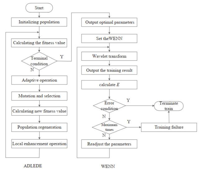
After the adaptive and local enhanced improvement of DE, the flow chart of ADDE is shown in Figure 2.
Figure 2 Flow chat of ADLEDE-WENN |
Full size|PPT slide
4 ADLEDE-WENN and the Comparative Forecasting Models
4.1 ADLEDE-WENN Forecasting Model
In ENN, gradient descent algorithm is usually chosen as the parameter learning algorithm, including the gradient descent (GD), the GDM, the Levenberg-Marquardt (LM) etc. But there is a vital defect of those algorithms, it is easy to fall into local optimum. Therefore, it is essential to find a new parameter adjustment method of the ENN. In this paper, we applied the ADDE algorithm to adjust the parameters of ENN. Based on the analysis mentioned above, the main steps of ADDE-WENN are described in Figure 2.
4.2 Comparative Models
To evaluate the effectiveness of the ADDE-WENN model in forecasting the closing price of the foreign exchange rates, other comparative models including ENN, WENN and ADDE-ENN are selected. ENN (described in Subsection 2.1) is the basic model, and other models are modified based on it. WENN was replaced the sigmoid function with wavelet function in the hidden layer based on ENN, and it was introduced in Subsection 2.3. ADDE-WENN refers to ADDE-ENN, which was researched in Subsection 4.1. To the transfer function of the hidden layer, the sigmoid function was used in ADDE-ENN, and the wavelet function was used in ADDE-WENN.
First, by comparing WENN with ENN, the effect of wavelet function to the Elman neural network could be studied. Second, by comparing ADDE-ENN with ENN, the feasibility and effectiveness of the ADDE algorithm could be evaluated in adjusting the parameters of the Elman neural network. Third, by comparing ADDE-ENN with ADDE-WENN, the effect of wavelet function could be researched on the use of ADDE to the Elman neural network. At last, in order to evaluate the comprehensive effects of the ADDE algorithm and the wavelet function to the Elman neural network, ADDE-WENN and ENN could be selected.
4.3 Performance Measure
In this part, we comparatively evaluate the prediction effects of wavelet function and ADDE algorithm applied to ENN. For further analyzing the forecasting performance of ENN, WENN, ADDE-ENN and ADDE-WENN, we choose several measures to value error and trend performance, including mean square error (MSE), mean absolute error (MAE), mean absolute percentage error (MAPE) and error limit proportion (ELP). Those are all the error-type measures of the deviation between predicted values and actual data, and those indexes reflect the prediction of global error. The corresponding definitions are given as follows:
Mean square error (MSE):
Mean absolute error (MAE):
Mean absolute percentage error (MAPE):
Error limit proportion (ELP):
where is the predict value and is the real value; denotes the number of the evaluated data; is the limited level. MSE, MAE and MAPE are the negative indexes. The smaller MSE, MAE and MAPE value show the less deviation of the forecasting results from the actual values. ELP is the positive index. The value of ELP is higher, and the accuracy is more precise.
5 Experiment Method
5.1 The Foreign Exchange Rate Data
In order to study the validity of the models, we selected 4 kinds of foreign exchange rate closing price. They were EURUSD, USDCNH, GBPUSD and GBPCNY, and the data was from Wind. The closing prices of EURUSD, USDCNH, GBPUSD were from the International Foreign Exchange Market (IFEM), and the closing price of GBPCNY was from the China Foreign Exchange Trade System (CFETS). The information of the foreign exchange rate was shown in Table 1.
Table 1 Foreign exchange information |
| Foreign exchange | Data | Beginning | End |
| EURUSD | IFEM | 2019.3.28 | 2020.2.26 |
| GBPCNY | CFETS | 2019.2.28 | 2020.2.26 |
| GBPUSD | IFEM | 2019.3.28 | 2020.2.26 |
| USDCNH | IFEM | 2019.3.28 | 2020.2.26 |
For each foreign exchange rate, 240 days of closing price were chosen. The data set was divided into the training and testing data set. The training data set was composed of 170 days in front, and it was accounting for 71% of the total data. The testing data set was composed of the rest 70 days accounting for 29% of the total data.
5.2 Normalization Preprocessing
The observed foreign exchange rate closing price is the non-normal data. Before we use the ANNs to predict the price, the price data should be normalized. In the data set, the minimum and the maximum values are used to normalize the data:
After the forecasting, anti-normalization need be used to obtain the true value by the formula:
where is the observed (anti-normalized) closing price; and are the minimum and the maximum prices of the data; is the normalized (predicted) data. In this paper, MSE is also applied to measure the performance of the ANNs models. We defined MSE and MSE* for different use. MSE was used to mark the result, in which the data was normalized. MSE* was used to mark the result, in which the data was anti-normalized.
5.3 Experimental Tools and Configuration of System
In this paper, Matlab was selected to implement those 4 models. To the Elman neural network, the neural network toolbox of MATLAB R2016a was used in the experiment, and the main parameters described in Table 2. While the ADDE algorithm was used in the experiment, the parameters of ADDE were set in Table 3.
Table 2 Parameters of Elman neural network |
| Parameters | Description | Value |
| M | Number of the input layer nodes | 5 |
| N | Number of the output layer nodes | 1 |
| K | Number of the hidden layer nodes | 10/12 |
| H | Number of the context layer nodes | 10/12 |
| transferFcn | Transfer function of the hidden layer | tansig/Morlet |
| trainFcn | Training function | traingdm |
| epochs | Maximum training times | 15, 000/1, 000* |
| Note: *1, 000 was set by using ADLEDE to the ANNs. Otherwise, it was set 15, 000. |
Table 3 Parameters of ADLEDE |
| Parameters | Description | Value |
| nofv | Number of the variables | 171/229* |
| lb | low bound of the variables | -1 |
| ub | up bound of the variables | 1 |
| popsize | population size | 100 |
| pl | the perturbation factor | 0.5 |
| LE | the local enhancement operator | 0.01 |
| the higher crossover probability | 0.8 |
| the lower crossover probability | 0.5 |
| the higher crossover factor | 0.09 |
| the lower crossover factor | 0.04 |
| Note: * When the hidden layer nodes were 10 (12), the variables were 171 (229). |
6 Results and Discussion
The data of the foreign exchange rate was described in Subsection 5.1, including EURUSD, GBPCNY, GBPUSD, and USDCNH. To study the performances of the models, which were ENN, WENN, ADDE-ENN and ADDE-WENN, all the 4 models were researched in the experiments to each group of the foreign exchange rate. There was a fatal defect to the ANNs——The randomness, which meant we couldn't get the same neural network exactly. The reason for the randomness was that: When the neural network was trained, the parameters to each of the neural network etc) were different. To reduce the impact of the randomness, each model was simulated 20 times in the experiment, and the result was the average value of all the 20 times. The results were shown in Table 4. Not all the figures of the experiments were shown in this paper, and part figures of EURUSD were shown in Figures 3~6.
Table 4 The results of the experiments |
| Measurement | Models | MSE* | | MAE | | MAPE(%) | | ELP-0.5%(%) |
| Training | Testing | Training | Testing | Training | Testing | Training | Testing | D-value* |
| EURUSD | ENN | 1.1783 | 1.4734e-5 | | 2.6632e-3 | 2.9016e-3 | | 0.2401 | 0.2583 | | 89.3529 | 85.4615 | -3.8914 |
| WENN | 2.5488e-5 | 5.1806e-5 | 3.8458e-3 | 5.0302e-3 | 0.3470 | 0.4466 | 76.8235 | 68.9231 | -7.9004 |
| ADDE-ENN | 9.5891e-6 | 1.2389e-5 | 2.3394e-3 | 2.6752e-3 | 0.2109 | 0.2381 | 91.4706 | 87.3846 | -4.0860 |
| ADDE-WENN | 9.3268e-6 | 1.0823e-5 | 2.2803e-3 | 2.5051e-3 | 0.2055 | 0.2230 | 92.2941 | 89.2308 | -3.0633 |
| GBPCNY | ENN | 2.6356e-3 | 2.1774e-3 | | 4.0411e-2 | 3.5434e-2 | | 0.4553 | 0.4023 | | 62.6765 | 70.4615 | 7.7850 |
| WENN | 7.4443e-3 | 4.0192e-3 | 6.3406e-2 | 4.9077e-2 | 0.7145 | 0.5576 | 47.4706 | 57.2308 | 9.7602 |
| ADDE-ENN | 1.9361e-3 | 1.9861e-3 | 3.4803e-2 | 3.1917e-2 | 0.3917 | 0.3623 | 67.8235 | 74.1538 | 6.3303 |
| ADDE-WENN | 1.9274e-3 | 1.9554e-3 | 3.4624e-2 | 3.1572e-2 | 0.3896 | 0.3584 | 68.1765 | 76.3077 | 8.1312 |
| ADDE-WENN* | 7.8462e-4 | 8.7937e-4 | 5.5716e-3 | 6.1457e-3 | 0.2486 | 0.2879 | 73.0534 | 81.4625 | 8.4091 |
| EURUSD | ENN | 5.2576e-5 | 2.5823e-5 | | 5.562e-3 | 4.0969e-3 | | 0.4385 | 0.3186 | | 66.2647 | 80.0015 | 13.7368 |
| WENN | 1.0515e-4 | 8.5562e-5 | 7.8274e-3 | 7.0712e-3 | 0.6177 | 0.5510 | 51.2941 | 57.8462 | 6.5521 |
| ADDE-ENN | 4.3148e-5 | 2.0371e-5 | 5.0465e-3 | 3.5886e-3 | 0.3980 | 0.2790 | 72.2353 | 85.3846 | 13.1493 |
| ADDE-WENN | 4.1936e-5 | 1.9777e-5 | 5.0064e-3 | 3.5425e-3 | 0.3949 | 0.2753 | 72.4706 | 85.8462 | 13.3756 |
| EURUSD | ENN | 6.2212e-4 | 4.9941e-3 | | 1.8443e-2 | 4.9553e-2 | | 0.2627 | 0.7338 | | 87.2647 | 56.0491 | -31.2156 |
| WENN | 1.4898e-3 | 3.0409e-2 | 2.9172e-2 | 11.0220e-2 | 0.4158 | 1.6330 | 69.6518 | 41.5385 | -28.1133 |
| ADDE-ENN | 4.8748e-4 | 4.8459e-3 | 1.5751e-2 | 1.9072e-2 | 0.2242 | 0.2810 | 91.6471 | 61.8462 | -29.8009 |
| ADDE-WENN | 4.8557e-4 | 6.3973e-4 | 1.5792e-2 | 4.4246e-2 | 0.2248 | 0.6555 | 91.8824 | 84.1372 | -7.7452 |
| Note: D-value* = Testing value − Training value;
ADLEDE-WENN* marks the structure of the neural network was changed. The numbers of the hidden and context layer nodes increased from 10 to 12. |
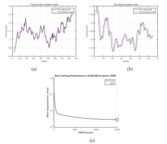
Figure 3 Forecasting EURUSD with ENN |
Full size|PPT slide
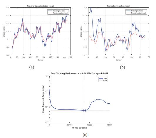
Figure 4 Forecasting EURUSD with WENN |
Full size|PPT slide
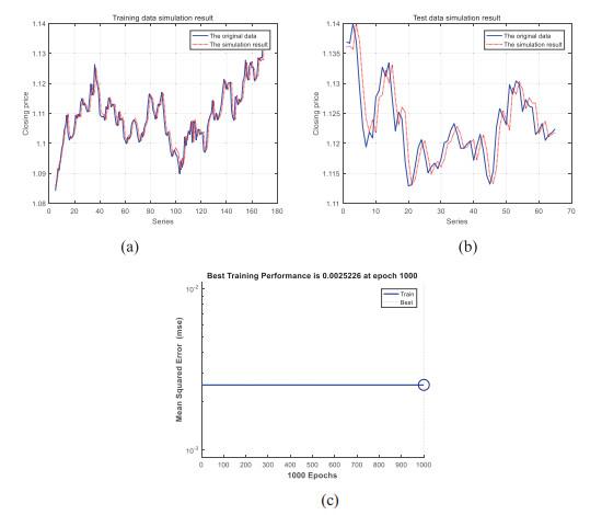
Figure 5 Forecasting EURUSD with ADLEDE-ENN |
Full size|PPT slide
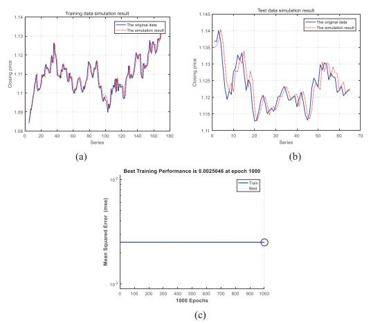
Figure 6 Forecasting EURUSD with ADLEDE-WENN |
Full size|PPT slide
6.1 The Impact of Wavelet Function to ENN
If the wavelet (Morlet) function was used in ENN, the efficiency of the traditional learning method (GDM in this paper) was decreased a lot. In the experiments of ENN and WENN, the training function was set as the "traingdm" which referred to the GDM. According to the result in Table 4, all the negative indexes (MSE*, MAE and MAPE) values of WENN were higher and the positive index (ELP-0.5%) was lower than the results of ENN to the same foreign exchange rate. The MSE of ENN and WENN was described in Figure 3(c) and Figure 4(c). MSE decreased smoothly in Figure 3(c), and it got the minimum value 2.7284 at the maximum time 15, 000. However, MSE was fluctuating in Figure 4(c), and it got the minimum value 5.6847 at 8, 669 times. Therefore, we could conclude that the wavelet function in the WENN disrupted the convergence of the traditional learning algorithm. The "disruption problem" was caused by the non-linear performance of the wavelet function. Therefore, in the experiments of WENN, it didn't improve the performance of ENN. However, the results were getting worse in reverse.
To evaluate the effect of a wavelet function, the ADDE algorithm was applied to both of ENN (ADDE-ENN) and WENN (ADDE-WENN). The performance of ADDE was described in Subsection 6.2. According to Table 4, the negative indexes value (MSE*, MAE and MAPE) of ADDE-ENN was higher and the positive index (ELP) was lower than the value of ADDE-WENN to the same foreign exchange rate. Comparing the experiments of ADDE-ENN and ADDE-WENN, the only difference was the transfer function in the hidden layer. The transfer function of ADDE-WENN was the wavelet (Morlet) function, and the sigmoid function was for ADDE-ENN. So, we could conclude that the differences in the result of the experiment were caused by the wavelet function. According to the testing result of EURUSD, the MSE, MAE and MAPE values of ADDE-WENN decreased by 12.64%, 6.36% and 6.34%, and the value of ELP-0.5% increased by 1.85%.
6.2 The Performance of the ADDE Algorithm
Based on the analysis of Subsection 6.1, it was necessary to adopt a new parameter training method in the WENN, which would give full play to the non-linear performance of wavelet function. The ADDE algorithm, which had the characters of fast convergence and global optimization capability, was applied to train the parameters of the neural network in the experiments.
The performance of the ADDE algorithm was researched by comparing ENN and ADDE-ENN. According to Table 4, the negative indexes value (MSE*, MAE and MAPE) of ENN was higher and the positive index (ELP-0.5%) was lower than the value of ADDE-ENN to the same foreign exchange rate. Comparing the experiments of ENN and ADDE-ENN, the difference was that the ADDE algorithm was used to train the parameters of the neural network in ADDE-ENN. According to the testing result of EURUSD, the MSE*, MAE and MAPE values of ADDE-ENN decreased by 15.92%, 7.80% and 7.82%, and the value of ELP-0.5% increased by 1.92%.
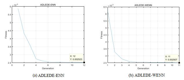
The performance of the ADDE algorithm was also researched by comparing ADDE-ENN and ADDE-WENN. In the training process of ADDE, the fitness values (MSE) of ADDE-ENN and ADDE-WENN were shown in Figure 7. In the experiment of ADDE-ENN, the ADDE algorithm terminated at 12 generations and got the optimal result 2.523. In the experiment of ADDE-WENN, the ADDE algorithm terminated at 11 generations and got the optimal result 2.507. The parameters were trained by the ADDE algorithm at first. Then, the parameters were sent to the neural network and trained by the traditional algorithm (GDM). According to Figure 5(c) and Figure 6(c), the MSE of ADDE-ENN was 2.5226, and the MSE* of ADDE-WENN was 2.5046. After 1, 000 times trained by the traditional learning algorithm, the MSE of both neural networks had limited improvement. Therefore, we concluded that it was effective to apply the ADDE algorithm to train the parameters of the neural network. After the training process of the ADDE algorithm, it almost got the global optimal solution. The traditional algorithm of the Elman neural network had limited performance to the forecasting result. ADDE algorithm could be applied to train the parameters of the neural network. In our experiments, it not only solved the "disruption problem" caused by the wavelet function, but also could take advantage of the non-linear characters belonging to wavelet function. By applying the ADDE algorithm to WENN, the forecasting performance of the neural network improved a lot.
Figure 7 The fitness (MSE*) of ADLEDE |
Full size|PPT slide
According to the testing results of EURUSD, GBPCNY, GBPUSD and USDCNH, all the indexes show that: ADDE-WENN ADDE-ENNENN ("" means better than). ADDE-ENN ENN meant that the ADDE algorithm was an effective method to train the parameters of the neural network. ADDE-WENN ADDE-ENN meant that the wavelet (Morlet) function of the hidden layer improved the performance of the neural network.
6.3 The Structure of the Models and the Over-Fitting Problem
The structure of ENN had a significant impact on the performance of ENN, including the number of the input layer nodes, the hidden layer nodes and the context layer nodes and so on. In the experiments, the same structure was applied to forecast different foreign exchange rates, and the parameters were shown in Table 2. According to the testing results of ELP-0.5%, the structure suited for EURUSD (89.2308) GBPUSD (85.8462) USDCNH (84.1372) GBPCNY (81.4625). Therefore, the experiments show that the same neural network structure had a different performance to forecast the foreign exchange rate. In other words, we should select a certain structure, which could reflect the low of fluctuation to the foreign exchange rate, to predict the close price. In the ADDE-WENN experiment of GBPCNY (marked ADDE-WENN* in Table 4), if the numbers of the hidden and context layer nodes increased from 10 to 12, all the indexes including MSE*, MAE, MAPE and ELP-0.5% improved a lot.
The over-fitting problem is common in the neural network. It means the neural network performs well in the training process, but performs badly in the testing process. In the experiments of USDCNH, the over-fitting problems were very serious to ENN and ADDE-ENN. According to the results of MSE*, MAE, MAPE and ELP-0.5%, the performance of the neural network was very bad in the testing process. It meant that the trained neural network was failed. By comparing the D-value of ADDE-ENN and ADDE-WENN, if the testing value was less than training value, the absolute D-value decreased; if the testing value was greater than training value, the absolute D-value increased. According to the results, we could conclude that the over-fitting problem in ADDE-WENN was less serious than that in ADDE-ENN, and the "improvement" was also brought about by the wavelet function in the hidden layer of WENN.
7 Conclusion
In the present paper, the ADDE-WENN predicting model is established aim to forecast the fluctuations of the foreign exchange rate. Based on the experiments of EURUSD, GBPCNY, GBPUSD and USDCNH, the follows could be concluded:
Firstly, if the wavelet function was applied to be the transfer function in the hidden layer of ENN, the non-linear character of the wavelet function could improve the performance of ENN in forecasting. But it would decrease the efficiency of the traditional learning algorithm at the same time. So, a new parameter training algorithm was needed under the circumstances.
Secondly, it was a feasible and effective way to train the parameters of the neural network with the ADDE algorithm. When the ADDE algorithm was applied in WENN, it could solve the "disruption problem" and take advantage of the non-linear character belonging to wavelet function. In this way, the performance of the neural network could be improved a lot.
Thirdly, the structure of the neural network had a significant impact on the performance of the neural network. Different structures were needed to forecast the foreign exchange rates.
At last, the over-fitting problem was common in the application of neural networks. The application of wavelet function in the neural network was conducive to weaken the problem of over-fitting.
In the present paper, other problems needed to be studied. There were many other wavelet functions, and the Morlet function was studied in this paper. It was necessary to study the performance of other wavelet functions applied to the neural network. Considering the impact of the structure on the neural network, it was a new problem about how to find a suitable structure for each foreign exchange rate.
{{custom_sec.title}}
{{custom_sec.title}}
{{custom_sec.content}}
 PDF(769 KB)

 Figure 1 The network structure of ENN
 Table 1 Foreign exchange information


