1 Introduction
Since oil has been dominating the sources of the world energy and playing an critical role in economic activities and industrial production for several centuries, all countries in the world concentrate on oil reserve and pricing while market participants are active in investment and speculation in the oil market. The imbalance between supply and demand and the other various market factors produce effects on the oil prices changes caused by the different shock origins which may have diversified influence on macroeconomic indicators in different economies. Under such circumstance, it is critical to figure out that whether and how international oil price fluctuation could lead to the effects on the macroeconomics and what the policy makers and market participants could do to deal with these effects, and to provide some valuable policy implications.
Most researches about the international oil fluctuation focus on two aspects: The reason of the international oil price fluctuation and the influence of the oil price changes on the macroeconomy. In earlier researches, scholars put forward a point of view that the international oil price is mainly affected by supply factors and take the macroeconomic factors as exogenous, such that the research about the influence of the international oil price changes on the macroeconomic is limited to the oil price itself. Since Hamilton
[1] pointed out that the oil price hikes is the Granger cause of the recession of U.S. economy, the effects of oil price shocks on the macroeconomy have increasingly been analyzed in a number of studies, such as economic growth
[2-6], commodity price
[7], exchange rate
[8-10], stock index returns
[11-13] etc.
With the in-depth study on the dependence between the oil price and the economy, scholars find that oil price is born economical and affect the world economy conversely. Kilian
[14] proposed the Structural Vector Autoregression (SVAR) model with the global crude oil production, global real economic activity, and real oil prices to distinguish among different sources of oil shocks, and decomposed the effects on oil price into oil supply shocks, aggregate demand shocks and oil-specific demand shocks. This model provides a new thinking to analyze the effects of oil price on the macroeconomy. Apergis and Miller
[15] applied SVAR model to investigate the sample of eight countries and show how the structural oil price shocks affect the stock market return. Kilian and Park
[16] affiliated U.S. stock market return into the three-variable SVAR model and establish four-variables SVAR model to analyze the effect of the structural oil shocks on the U.S. stock market. Peersman and Robays
[17] use SVAR model to investigate the effects of structural oil price shocks on the macroeconomy of different industrial countries. Ji, et al.
[18] analyzed the influence of structural oil price shocks on production, exchange rate and inflation in BRICS countries. Li, et al.
[19] affiliated domestic demand shock into three-variable SVAR model to study how structural oil price shocks affect Chinese stock market return. However, the researches mentioned above all apply SVAR model to build the mean model and use the impulse response analysis and variance decomposition, and don't take the dynamic effects of the structural oil price on the economic variables into consideration. Furthermore, there exist some studies on the time-varying characteristics, for instance, Broadstock and Filis
[20] combined the SVAR model and the Scalar-BEKK model to investigate the relationship between structural oil price shocks and stock market returns. Aastveit, et al.
[21] and Baumeister and Peersman
[22] applied the time-varying parameter VAR model (TVP-VAR) to study the effect of the oil price shock on the macroeconomy. An alternative dynamic method is the DCC-GARCH model which is applied by Filis, et al.
[23] to analyze the dynamics between stock market returns of oil importing and exporting countries and the international oil price.
In this paper, we employ Kilian's SVAR model
[16] to decompose the international oil price shocks into oil supply shocks, aggregate demand shocks and oil-specific demand shocks. Then the DCC-GARCH model is used to investigate the dynamic relationship between these three oil shocks and macroeconomic indicators. Then to quantify the intensity of effects of oil shocks on these variables, we propose a new measure, conditional expectation (CoE) capturing the difference between the expected level of the macroeconomic variable conditional on the oil price shock and that conditional on the benchmark state of the oil price. Although the TVP-VAR model is useful to study the dynamic characteristics of the influence between two variables, it is not flexible to capture the different effect modes (e.g., CoE). In this paper we propose to use the time-varying copula (see [
24]) to character the joint distribution between the oil shocks and the macroeconomic variables, to estimate the proposed measure. As the proxy of the macroeconomy, we choose the industrial output, inflation and exchange rate which are usually considered as the main macroeconomic variables by most researchers, as well as the economic policy uncertainty. As argued by many scholars (see [
25-
28]), oil price increases driven by different kinds of oil shocks have different consequences on the U.S. economic policy uncertainty. In this study, we extend the focused objects to several main oil importing and exporting countries in the world.
The main contributions of this paper are as follows: 1) Combining SVAR model with DCC-GARCH model, we temporally study the dynamic correlation between oil price shocks and a country's macro-economy in different time periods from the perspective of structural impact of oil price, rather than just regarding the oil price as a variable born out of the global economy; 2) We propose a new measure, to quantify the intensity of effects of oil shocks on macroeconomic variables, estimated by the time-varying copula model; 3) From the perspective of oil importing and exporting countries, the spatially comparative analysis is carried out among the major economies in the world, and the commonness and differences between these countries are discussed.
The remainder of this paper is organized as follows. Section 2 outlines the methodology. Section 3 introduces the data for major oil importing and exporting countries along with some descriptive statistics. Section 4 presents empirical results and the final section concludes and gives some policy suggestion.
2 Methodologies
With the regard to the research methodology, we firstly apply the Kilian's SVAR model
[16] to decompose the oil price shocks into the oil supply shocks, aggregate demand shocks and oil-specific demand shocks. Then, the DCC-GARCH model is exploited to analyze the dynamic dependence between three kinds of oil shocks and macroeconomic variables of different economies. Finally, we apply the conditional expectation to analyze the dynamic impact of oil shocks on the macroeconomic indicators.
2.1 SVAR Model
Consider a VAR model based on the data
, where
is the percent changes in global crude oil production,
denotes the index of real economic activity, and
defers to the real price of the oil. Kilian's SVAR model
[16] is given by
where denotes the vector of serially and mutually uncorrelated structural innovations. We assume that has a recursive structure such that the reduced-form errors can be decomposed according to :
This model postulates a vertical short-run supply curve of crude oil. Changes of the demand curve caused by either of the two oil demand shocks leads to an immediate shifts in the real price of oil, as do unpredictable oil supply shocks that change the vertical supply curve. The limitations on may be motivated as follows.
Crude oil supply shocks are defined as unanticipated innovations to global production. It is assumed that crude oil supply does not respond to innovations to the demand for oil within the same month. Innovations to global real economic activity that cannot be explained based on crude oil supply shocks will be referred to as shocks to the global demand for industrial commodities, that is, the aggregate demand shocks. Furthermore, innovations to real price of oil that cannot be explained based on oil supply shocks or aggregate demand shocks by construction will reflect changes in the demand for oil as opposed to changes in the demand for all industrial commodities. The latter structural shock will reflect, in particular, fluctuations in precautionary demand for oil driven by uncertainty about future oil supply shortfalls. Whereas this shock potentially could also reflect other oil market-specific demand shocks, there are strong reason to believe that it effectively represents exogenous shifts in precautionary demand.
Firstly, there are no other plausible candidates for exogenous oil market-specific demand shocks. For instance, Asian consumers' preference for durable goods (such as automobiles) has increased since 2003, leading to a sharp rise in real oil prices. This preference may seem to be an exogenous special demand shock. However, the rise in oil prices is not associated to the rise of oil-specific demand, but is caused by global economic prosperity, allowing us to exclude this interpretation.
Secondly, the empirical results of Kilian
[16] show that the large impact effect of the oil-specific demand shock is very different from those caused by other factors.
Thirdly, the timing of these oil-specific demand shocks and the direction of their effects is in accordance with the timing of exogenous events such as the outbreak of the Persian Gulf War that would be expected to affect uncertainty about future oil supply shortfalls on a priori grounds.
Fourthly, the movements in the real price of oil induced by this shock are highly correlated with independent measures of the precautionary demand component of the real price of oil based on futures prices. Applying oil futures market data, Alquist and Kilian
[29] show that this correlation may be as high as 80 percent, notwithstanding the use of a completely different dataset and methodology.
2.2 DCC-GARCH Model
Bollerslev
[30] proposes constant conditional correlation GARCH model (CCC-GARCH) shown as follows:
Let denote random variables with mean equal to 0 and satisfy:
where denotes conditional covariance matrix given as follows:
where , denotes the matrix of conditional correlation coefficients which are constants. denotes the conditional variance characterized by an univariate GARCH model given as follows:
Although CCC model can simplify the calculation of variance matrix, the assumption that the correlation coefficient between assets is constant does not conform to the reality. For this reason, Engle
[31] introduced the DCC-GARCH model, assuming that the correlation coefficients are time-varying, and showing this model's advantage in parameter estimation. Specifically, the mean equation of DCC model is the same as Equation (3)
(5) while the residual equation (6) is replaced by
where , denotes the dynamic, time-varying matrix of conditional correlation coefficient with the dynamic constraint
where , denotes unconditional correlation matrix of standardized residual. Obviously, the matrix to be positive definite or positive semi-definite is a sufficient condition for the to be positive definite. and are coefficients of the DCC-GARCH model.
2.3 Conditional Expectation Model
Conditional expectation (CoE) for the macroeconomic variable is the expectation of the distribution of the macroeconomic variable, conditional on the fact that a given oil price shock occurs. Let be the values of the macroeconomic variable and be the values of the oil price shock. For the oil supply shock, decrease means the global oil supply declines. For the aggregate demand shock and the oil-specific demand shock, increase means the oil demand rises. Then, the "shock" can be defined by falling below some threshold for the oil supply shock or rise above some threshold for both demand shocks. For simplified and unified computation, we use the sign-opposite value of sequences for both aggregate demand shocks and oil-specific demand shocks. These three kinds of "shocks" can be all defined as , where is the -quantile as the threshold. The conditional distribution of the macroeconomic variable is defined as follows:
and the conditional expectation (CoE) of can be calculated by
An alternative method to calculate the conditional distribution shown as Equation (11) is copula function if we express this equation as
where and are marginal distributions of and , respectively. is the copula function linking both marginal distributions. Given a specific copula function, the conditional expectation (CoE) in Equation (12) can be calculated.
We denote the intensity of effects of the oil shock on the macroeconomic variable by
where means oil supply or demand are in the median state. Hence, can capture the percentage difference between the expected level of the macroeconomic variable conditional on the oil price shock and the expected level of the macroeconomic variable conditional on the benchmark state of the oil price.
Considering that there could exist negative, positive, and tail dependence between the oil price shock and the macroeconomic variable, we link both two marginal distributions by the Student's copula specified as:
where
denotes the dependence parameter and
denotes the degree of freedom. In addition, we consider possible time-varying parameter dependence by allowing the parameter to vary according to a specific evolution equation, which is the ARMA
type process (see [
24]) as follows:
where is the modified logistic transformation that keeps the value of in . The dependence parameters are explained by constants, an autoregressive term, and the average product over the last observations of the transformed variables.
3 Data Description
As for countries to be investigated, the selection criteria consist of that monthly macroeconomic data is available, and that the selected countries should be the top 20 oil importers or exporters in the world, and are the major economies that have an important impact on the world economy. Based on these two points, we choose China, U.S., Japan and India as the oil importers, and Brazil, Canada and Russia as the oil exporters. In importing countries, China's degree of dependence on international crude oil in 2016 was 64.5%, U.S.'s degree of dependence on international crude oil in 2015 was 42.5%, Japan's in 2015 was 99.7% and India's in 2014 was 70%. Obviously, our selected importing countries all have a high degree of dependence on international crude oil and their economies is more likely to be influenced by international crude oil price changes.
As for the macroeconomic variables, the selection criteria consist of that the chosen variable should be an important indicator of the macroeconomic situation of an economy (e.g., production, exchange rate, interest rate) and that the monthly data of these chosen variables is available. Based on this two points, we choose industrial output, economic policy uncertainty, inflation and exchange rate as macroeconomic variables.
The monthly data of selected variables consist of two parts: One is the international oil market data, the other is the macroeconomic indicator data of different countries. As for the international oil market, we refer to Kilian's selection: Global crude oil production (OPROD), global economic activity (EACT), international oil price (OP). As for macroeconomic variables, we choose industrial output index (IOI), economic policy uncertainty (EPU), inflation (Customer Price Index, CPI), exchange rate (EXR). The variables are prefixed by the name of the country to represent the macroeconomic variables of different countries.
Global crude oil production data is collected from the US Energy Information Agency (EIA,
http://www.eia.gov/). We take the Global Dry Bulk Rate Index proposed by Kilian
[16] as the proxy of the variable EACT. The reason of GDP or the weighted increment of the industrial production of these countries are not chosen is that the disclosure of GDP is generally lagging, the cycle is larger, even many countries have no monthly disclosure of GDP. Based on Dry Cargo Bulk Freight Rates Kilian
[16] proposed the Global Dry Bulk Rate Index, which contains more dynamic information and has significant positive correlation with economic activity so as to reflect the situation of global economic activity. This index can be collected from Kilian's website (
http://www-personal.umich.edu/~lkilian/). Furthermore, Brent crude oil price are considered as the proxy of the global international oil price (OP) because its covering about 60 percent share of the crude oil trade and can be collected from the U.S. Energy Information Agency (EIA).
As a proxy of industrial output index (IOI), we use the gross industrial production for U.S. and Canada, the industrial added values on a year-on-year basis for China (see [
19]), the industrial production index for Japan, India, Russia and Brazil. These data are collected from WIND database. The economic policy uncertainty (EPU) can be measured by Economic Policy Uncertainty index proposed by Baker, et al.
[32] based on the frequency of the news reports to measure the changes of the economic uncertainty relevant with the policy. For instance, as they show, the US EPU index has peaks in the presidential election, the first and second Gulf wars, the 911 attacks, the Lehman Brothers bankruptcy, the 2011 European debt crisis and other major fiscal policy events (for the EPU index of the major countries in the world, see
http://www.policyuncertainty.com/index.html). As a proxy of inflation, we use the Consumer Price Index (CPI) collected from the WIND database. As a proxy of exchange rate (EXR), we use real effective exchange rate index collected from Bank of international settlements.
Apart from Indian economic policy uncertainty index whose available data interval is relatively short (from January 2003 to December 2016), the sample interval of all other countries is from January 2000 to December 2016, including 204 observations for each variable (Indian EPU variable includes 168 observations). Many studies have focused on the three oil crisis in twentieth Century and the global financial crisis in 2008, while there are few studies on the price of oil in recent years. The sample interval of this article allows us to study the impact of oil prices on the macro-economy after 2008, filling the timeliness and completeness of the gaps and shortcoming.
Following the treatment of Kilian
[16], apart from the crude oil production (OPROD) using the returns, all other variables use the raw data. Considering the stationary of the data sequence, we use the first order difference of all series to ensure the stability of the fitted SVAR model.
Table 1 reports some basic descriptive statistics about all series in our sample.
Table 1 Descriptive statistics of the sample series |
| | Variable | Mean | Max | Min | Std.Dev | Skew. | Kurt. | JB stat. | -value |
| Global | OPROP | 0.14 | 2.62 | 2.46 | 0.76 | 0.17 | 4.12 | 11.67 | 0.0029 |
| EACT | 6.85 | 66.36 | 133.65 | 33.64 | 0.57 | 3.80 | 16.55 | 0.0003 |
| OP | 64.79 | 132.72 | 18.71 | 32.31 | 0.34 | 1.79 | 16.40 | 0.0003 |
| China | CH_IOI | 12.41 | 29.20 | 2.93 | 4.76 | 0.01 | 3.13 | 0.15 | 0.9285 |
| CH_EPU | 136.71 | 646.91 | 9.07 | 94.25 | 1.99 | 8.81 | 420.66 | 0.0000 |
| CH_CPI | 100.20 | 102.60 | 98.40 | 0.66 | 0.22 | 3.50 | 3.76 | 0.1523 |
| CH_EXR | 100.90 | 131.01 | 81.89 | 13.81 | 0.70 | 2.40 | 19.58 | 0.0001 |
| U.S. | US_IOI | 3488.48 | 3750.79 | 3137.32 | 144.74 | 0.15 | 2.11 | 7.47 | 0.0239 |
| US_EPU | 113.85 | 245.13 | 57.20 | 36.99 | 0.77 | 2.94 | 20.13 | 0.0000 |
| US_CPI | 209.14 | 241.73 | 168.80 | 22.38 | 0.19 | 1.67 | 16.41 | 0.0003 |
| US_EXR | 108.84 | 128.93 | 93.15 | 9.96 | 0.30 | 2.00 | 11.57 | 0.0031 |
| Japan | JA_IOI | 101.41 | 125.30 | 73.50 | 9.10 | 0.03 | 3.38 | 1.27 | 0.5305 |
| JA_EPU | 106.05 | 239.81 | 48.38 | 33.20 | 1.11 | 4.92 | 73.28 | 0.0000 |
| JA_CPI | 97.71 | 100.40 | 95.70 | 1.28 | 0.64 | 2.22 | 19.10 | 0.0001 |
| JA_EXR | 95.50 | 128.09 | 68.19 | 14.59 | 0.06 | 2.42 | 2.97 | 0.2268 |
| India | IN_IOI | 134.69 | 198.70 | 73.00 | 39.18 | 0.24 | 1.55 | 19.84 | 0.0000 |
| IN_EPU | 98.11 | 283.69 | 24.94 | 53.75 | 1.14 | 4.12 | 45.16 | 0.0000 |
| IN_CPI | 509.91 | 878.00 | 299.00 | 193.36 | 0.57 | 1.85 | 22.43 | 0.0000 |
| IN_EXR | 93.91 | 104.77 | 84.24 | 4.70 | 0.48 | 2.47 | 10.26 | 0.0059 |
| Brazil | BR_IOI | 91.11 | 112.60 | 65.33 | 10.95 | 0.06 | 2.13 | 6.63 | 0.0363 |
| BR_EPU | 139.45 | 473.53 | 22.30 | 77.31 | 1.78 | 6.89 | 236.34 | 0.0000 |
| BR_CPI | 3012.79 | 4940.78 | 1598.24 | 908.36 | 0.35 | 2.29 | 8.61 | 0.0135 |
| BR_EXR | 78.34 | 110.15 | 42.07 | 16.37 | 0.16 | 2.06 | 8.36 | 0.0153 |
| Canada | CA_IOI | 48068.49 | 53668.07 | 38330.99 | 2956.46 | 0.87 | 3.52 | 27.96 | 0.0000 |
| CA_EPU | 135.32 | 442.37 | 39.32 | 76.87 | 1.15 | 4.39 | 61.36 | 0.0000 |
| CA_CPI | 112.80 | 129.10 | 93.50 | 10.18 | 0.13 | 1.83 | 12.23 | 0.0022 |
| CA_EXR | 89.47 | 106.80 | 71.81 | 9.69 | 0.24 | 1.75 | 15.09 | 0.0005 |
| Russia | RU_IOI | 95.30 | 127.50 | 64.60 | 14.83 | 0.39 | 2.24 | 10.16 | 0.0062 |
| RU_EPU | 118.96 | 370.51 | 12.40 | 71.61 | 1.15 | 4.17 | 56.60 | 0.0000 |
| RU_CPI | 100.88 | 103.85 | 99.59 | 0.66 | 1.33 | 5.33 | 106.66 | 0.0000 |
| RU_EXR | 85.07 | 110.61 | 47.49 | 16.43 | 0.27 | 1.88 | 13.10 | 0.0014 |
| Notes: Std.Dev, Skew., Kurt., and JB stat. denote standard deviation, skewness, kurtosis and JB statistics, respectively. |
From Table 1, we can find that Jarque-Bera tests reject the null Gaussian distribution for all the series under 0.05 confidence level, except for China industrial output, China CPI, Japan industrial output, Japan real exchange rate, which shows the evidence that the distributions of most series are not normal.
The establishment of the SVAR model and the DCC model requires that all the time series are stationary and have the ARCH effects. Through ADF test and ARCH-LM test as shown in
Table 2, we find that all series are stationary and that international oil market and most of the macroeconomic variables have ARCH effects. Though the economic policy uncertainty, inflation and real exchange rate in some countries do not passed by test, referring to Li, et al.
[19], we still keep these variables for consideration of the integrity of this research.
Table 2 Unit root test and ARCH effects test for all series |
| | Variable | ADF | -value | ARCH-LM | -value |
| Global | OPROP | 12.03 | 0.0000 | 3.86 | 0.0024 |
| EACT | 10.51 | 0.0000 | 9.05 | 0.0000 |
| OP | 9.49 | 0.0000 | 10.15 | 0.0000 |
| China | CH_IOI | 13.23 | 0.0000 | 6.77 | 0.0000 |
| CH_EPU | 14.47 | 0.0000 | 19.61 | 0.0000 |
| CH_CPI | 12.63 | 0.0000 | 2.66 | 0.0238 |
| CH_EXR | 10.12 | 0.0000 | 0.87 | 0.5012 |
| U.S. | US_IOI | 3.66 | 0.0271 | 15.42 | 0.0000 |
| US_EPU | 12.75 | 0.0000 | 0.56 | 0.7310 |
| US_CPI | 9.08 | 0.0000 | 4.11 | 0.0015 |
| US_EXR | 10.30 | 0.0000 | 0.48 | 0.7894 |
| Japan | JA_IOI | 5.06 | 0.0002 | 4.15 | 0.0013 |
| JA_EPU | 12.82 | 0.0000 | 2.87 | 0.0159 |
| JA_CPI | 11.76 | 0.0000 | 0.14 | 0.9817 |
| JA_EXR | 10.87 | 0.0000 | 2.09 | 0.0679 |
| India | IN_IOI | 3.52 | 0.0406 | 7.89 | 0.0000 |
| IN_EPU | 16.11 | 0.0000 | 21.45 | 0.0000 |
| IN_CPI | 7.21 | 0.0000 | 0.43 | 0.6120 |
| IN_EXR | 13.07 | 0.0000 | 0.06 | 0.8935 |
| Brazil | BR_IOI | 3.89 | 0.0141 | 3.66 | 0.0019 |
| BR_EPU | 9.94 | 0.0000 | 4.38 | 0.0008 |
| BR_CPI | 6.08 | 0.0000 | 1.36 | 0.2431 |
| BR_EXR | 9.84 | 0.0000 | 5.52 | 0.0001 |
| Canada | CA_IOI | 14.88 | 0.0000 | 9.49 | 0.0000 |
| CA_EPU | 11.11 | 0.0000 | 1.47 | 0.2017 |
| CA_CPI | 11.23 | 0.0000 | 0.72 | 0.6077 |
| CA_EXR | 11.09 | 0.0000 | 1.74 | 0.0752 |
| Russia | RU_IOI | 3.19 | 0.0892 | 2.70 | 0.0221 |
| RU_EPU | 12.94 | 0.0000 | 5.79 | 0.0001 |
| RU_CPI | 5.76 | 0.0000 | 4.03 | 0.0462 |
| RU_EXR | 3.59 | 0.0335 | 11.46 | 0.0000 |
4 Empirical Results
In this section, first we apply impulse response function to analyze the impact of structural oil price shocks on macroeconomic variables for each country. Then we empirically investigate dynamic dependence between structural oil price shocks and macroeconomic variables using the monthly observations of the international crude oil market and the macroeconomic variables in different countries. Finally, the dynamic impact of oil price shocks on macroeconomic variables are calculated by applying the measure of the impact intensity, , described in Section 2.3.
4.1 The Impact of Structural Oil Price Shocks on Macro-Economy
The underlying causes of oil price increases are decomposed into three kinds of shocks in this work. Oil supply shocks are defined as unpredictable interruptions to global oil production; aggregate demand shocks represent innovations in the oil flow demand induced by a global economic boom; and oil-specific demand shocks are innovations in crude oil prices and mainly caused by expectation changes or speculative activities in global oil markets. It can be expected that the influence of these shocks on the macroeconomic indicators of each oil-importing and exporting country will be quite different because of their different transmission paths.
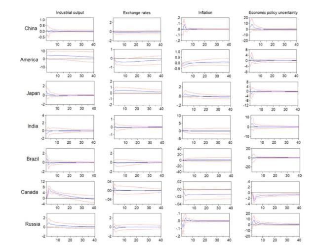
The oil supply shock is the oil price increasing caused by the shortage of global oil supply. The main source is the interruption of global oil production, such as war, weather, production limit of exporting countries etc. The impacts of one negative standard deviation oil supply shock on industrial output, exchange rates, inflation, and economic policy uncertainty for each country are shown in Figure 1. Then, the positive response means oil supply disruptions will increase the macroeconomic indicator, which is different from aggregate demand shocks and oil-specific demand shocks. The significance of impulse response function is defined as both one-standard-error bands are above or below zero on the -axis.
Figure 1 Response of industrial output, exchange rates, inflation, and economic policy uncertainty to oil supply shocks |
Full size|PPT slide
From
Figure 1, we can find that effects of oil supply shocks on oil importing countries are not almost significant, such as China, America, Japan, and India. The insignificant responses of China and India may be mainly due to that these two countries are still in an early stage of industrialization and coal has a dominant role in their energy structure as mentioned by Ji, et al.
[18]. The insignificant responses of America and Japan may be because these two countries are developed economies and have relatively complete oil reserve system. Moreover, impacts of oil supply shocks on industrial output, inflation, and economic policy uncertainty of oil exporting countries are advantageous, such as Russia and Canada. This is expected because the oil price rise caused by oil supply shortage is conducive to the oil exporters directly. However, the responses of Brazil's macroeconomic variables are almost not significant, which may be attributed to its increasing amount of biomass consumption in both the residential and industrial sectors.
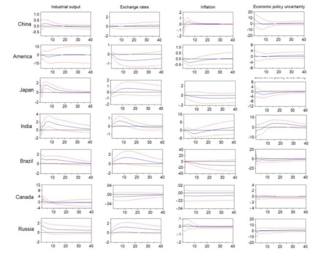
The global aggregate demand shock can be represented by the oil price rise caused by global economic prosperity. This shock played an important role in the rise of oil price in 2000–2008. In theory, the rise of the oil price caused by the global aggregate demand shock can be predicted and the degree of this shock is significantly different from that of the oil supply shock because of the canceling effect of the oil price rising and the global economic growth.
Different from oil supply shocks, aggregate demand shocks have more significant effects on oil importing countries than oil exporting countries as shown in Figure 2. For instance, the industrial output of Japan and India show positive responses to aggregate demand shocks because of the global economic expansion. During the economic prosperity, emerging countries' exchange rates tend to appreciate response to global aggregate demand shocks (e.g., India, Brazil, and Russia) more than developed economies (e.g., America and Canada) because emerging countries could experience more high-speed economic growth. In addition, responses of China's macroeconomic variables to aggregate demand shocks are still not significant, which may be due to the neutralization effect between aggregate demand shocks and economic expansion and Chinese government's macro-control policies of monetary and price. Response of economic policy uncertainty of both oil importing countries and exporting countries to aggregate demand shocks are almost not significant excluding India (positive response after about one year), which indicates that India's economy may experience a period of instability after the economic prosperity.
Figure 2 Response of industrial output, exchange rates, inflation, and economic policy uncertainty to aggregate demand shocks |
Full size|PPT slide
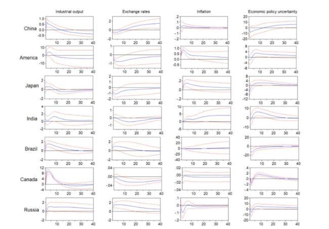
The oil-specific demand shock mainly refers to the oil reserve demand caused by the fear of the future oil supply shortage and the speculative demand generated from the expectation of the future oil supply shortage. This demand is mainly from the uncertainty of the oil price.
From Figure 3, we can find that oil-specific demand shocks have more significant effects on macroeconomic variables of both oil importing and exporting countries than oil supply shocks and aggregate demand shocks in general, particularly for China, America, and Japan. For China, the response of industrial output to the oil price uncertainty change from positive to negative after one year and real exchange rate from negative to positive at the same time, which shows that oil-specific demand shocks will slowdown China's industrial growth and increase its real exchange rates in the future. The significant responses of America's real exchange rates and inflation and insignificant response of its industrial output show that as a mature industrialized country, America's financial system is more directly affected than industrial system by the oil price uncertainty, as well as Japan. Similar with oil supply shocks, oil-specific demand shocks will benefit oil exporting countries directly considering the oil-export rise caused by either the industrial production or the energy strategic reserve of oil importers. Moreover, responses of economic policy uncertainty of both importers and exporters to oil-specific demand shocks are almost positively significant in the short- or long-term excluding Brazil.
Figure 3 Response of industrial output, exchange rates, inflation, and economic policy uncertainty to oil-specific demand shocks |
Full size|PPT slide
4.2 The Dynamic Dependence Between Structural Oil Price Shocks and Macro- Economy
4.2.1 Oil Supply Shocks and Macro-Economy
This shock differs from the other two shocks and the oil supply decline will cause the oil price to rise. Therefore, the positive correlation between oil supply and some macroeconomic variable implies that oil supply decline and the oil price rise cause this macroeconomic variable to decline, and the negative correlation indicates that the oil supply decline and the oil price rise cause this macroeconomic variable to rise.
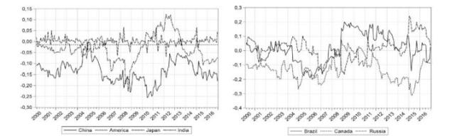
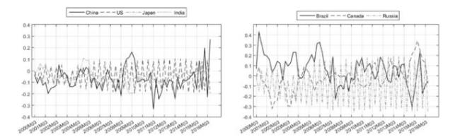
Table 3 shows the mean value of dynamic correlation sequence between the oil supply shock and the macroeconomic variable we obtain empirically. Figures 14 show that the dependence between oil supply shock and macroeconomic variables of oil import and export countries exhibit obvious dynamics.
Table 3 Mean value of dynamic correlation sequence between the oil supply shock and the macroeconomic variables |
| | Importers | | Exporters |
| China | U.S. | Japan | India | Brazil | Canada | Russia |
| IOI | 0.00 | 0.16 | 0.06 | 0.44 | | 0.19 | 0.24 | 0.21 |
| EPU | 0.17 | 0.27 | 0.06 | 0.14 | 0.22 | 0.44 | 0.09 |
| CPI | 0.70 | 0.16 | 0.30 | 0.15 | 0.01 | 0.73 | 0.06 |
| EXR | 0.04 | 0.36 | 0.37 | 0.16 | 0.08 | 0.00 | 0.10 |
Figure 4 Dynamic dependence between oil supply shock and IOI of importers and exporters |
Full size|PPT slide
As for the industrial output, Table 3 shows the evidence that Indian industrial output is negatively dependent with the oil supply shock, which means Indian industrial output increases with the oil price rising caused by the shortage of the oil supply. This may be due to the ongoing industrialization of India as an emerging market. Coal is still the main energy source of its industrial production, which accounts for 53% of total energy consumption, thereby reducing the impact of oil supply shocks, which is consistent with the results obtained by the impulse response in Subsection 4.1.1. From Figure 4, we can find that most of the time series exhibit time-variation. Specifically, the weak negative correlation (almost 0) between oil supply shock and industrial output in Japan and China become positive and stronger after the financial crisis in 2008, which implies oil price shocks caused by the shortage of the short-run oil supply contribute to the decrease of the industrial output in Japan and China. Moreover, the correlation sequence of Russia shows obvious time-variation, particularly at the time points of the oil price fluctuation in 2008, 2011 and 2014.
As for the economic policy uncertainty, as a whole, in the importing countries, the United States, Japan and India show weak negative correlation in addition to the weak positive correlation of China as shown in Table 3. This signifies that for importing countries, the shortage of international oil supply generally cause the economic policy uncertainty increasing, which goes against the domestic economic stability. Generally speaking, because of the strong dependence of the importing countries on the supply of international oil, the shortage of the oil supply may lead to economic panic. In the exporting countries, Brazil shows weak negative correlation while Canada and Russia exhibit positive correlation, but weak for Russia. This result accords with the general understanding, because the international oil supply shortage is a good news for the exporting countries, whether the rise in oil prices leading to more export income, or the opportunity to increase production to expand market share, or obtaining more right of oil pricing, are very beneficial to the economic stability of the exporting countries. For the importing countries, as shown in Figure 5, the effects of oil supply shocks on the economic policy uncertainty are weak and the duration of the effects caused by some temporary special event. During the global financial crisis in 2008, the correlations of four countries all appeared short-term fluctuations. The positive or negative correlations all shocked to zero in short term while the correlation of China changed from positive to negative in a short period of time. This indicates that the impact of oil supply shocks on importing countries decrease during the financial crisis, which is logical, because oil-specific demand shocks play a leading role in the financial crisis. The correlations of China and the United States were strengthened transitorily for the national turmoil of part Arabia in 2011, which was a manifestation of the increase in the impact of supply.
Figure 5 Dynamic dependence between oil supply shock and EPU of importers and exporters |
Full size|PPT slide
As for the inflation, Table 3 shows that correlations between the oil supply shock and the inflation of a country are negative excluding Japan and Russia, which indicates that the rise of the oil price caused by the oil supply shortage will result in the cost-push inflation existing in both importing and exporting countries. In general, as the industrial energy and chemical raw materials, oil becomes irreplaceable for both importing and exporting countries and the increase of its price will lead to the rising prices for the whole society. Moreover, the oil exporters considered in this paper are large countries not only exporting oil but also having international economic status, rather than the Middle East countries whose main economic support is oil industry. The negative correlation between oil supply shocks and their inflation is reasonable. It is worth noting that the relative strong negative correlations of China and Canada show the evidence that the inflation of both countries could be affected significantly by the international oil supply shocks. Therefore, the governments should be vigilant and formulate and improve the policies of oil reserve strategy and price stabilization against the impact of oil supply shocks on domestic commodity prices. From Figure 6, we can find that the fluctuation trend of the correlations of these countries turn to be negative in 2008, which shows that after the financial crisis the inflation caused by the oil supply shocks has increased in the short term. However, the global aggregate demand shocks played a leading role in this period, so the increasing degree is not very obvious.
Figure 6 Dynamic dependence between oil supply shock and CPI of importers and exporters |
Full size|PPT slide
As for the exchange rate, Table 3 shows the significantly negative correlations of U.S. and Japan and the weak correlations for others, which indicates that the dependence between oil supply shocks and the exchange rate is weak for oil exporting countries and is negative for most oil importing countries, particularly for U.S. and Japan. As shown in Figure 7, the shift of the correlations of U.S. and Japan is little while that of China and India is large because the emerging markets may be more volatile to various factors. Furthermore, in importers, the time-varying correlations of U.S., Japan and India are smaller than zero while that of China is almost lager than and close to zero, which indicates that at most of the time oil supply shock will bring a slight decline in China's real effective exchange rate index and a slight devaluation of the RMB. This shows that China should be more vigilant against the oil supply shocks than other importing countries, but it will not affect the RMB exchange rate basically.
Figure 7 Dynamic dependence between oil supply shock and EXR of importers and exporters |
Full size|PPT slide
4.2.2 Aggregate Demand Shocks and Macro-Economy
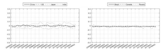
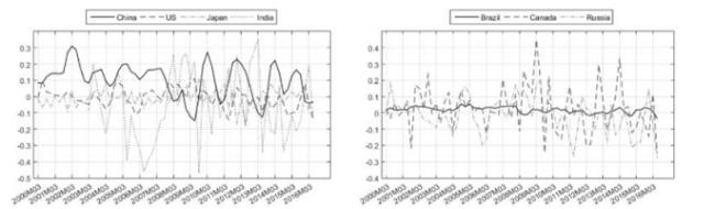
Table 4 shows the mean value of dynamic correlation sequence between the global aggregate demand shock and the macroeconomic variable we obtain empirically. Figures 811 show that the dependence between global oil aggregate demand shock and macroeconomic variables of oil import and export countries exhibit obvious dynamics.
Table 4 Mean value of dynamic correlation sequence between the aggregate demand shock and the macroeconomic variables |
| | Importer | | Exporter |
| China | U.S. | Japan | India | Brazil | Canada | Russia |
| IOI | 0.04 | 0.13 | 0.08 | 0.02 | | 0.11 | 0.08 | 0.11 |
| EPU | 0.60 | 0.23 | 0.44 | 0.03 | 0.32 | 0.21 | 0.11 |
| CPI | 0.13 | 0.28 | 0.34 | 0.11 | 0.24 | 0.20 | 0.02 |
| EXR | 0.03 | 0.04 | 0.26 | 0.02 | 0.01 | 0.18 | 0.06 |
Figure 8 Dynamic dependence between aggregate demand shock and IOI of importers and exporters |
Full size|PPT slide
Figure 9 Dynamic dependence between aggregate demand shock and EPU of importers and exporters |
Full size|PPT slide
Figure 10 Dynamic dependence between aggregate demand shock and CPI of importers and exporters |
Full size|PPT slide
Figure 11 Dynamic dependence between aggregate demand shock and EXR of importers and exporters |
Full size|PPT slide
As for the industrial output, as shown in Table 4, the dependence between global oil aggregate demand shocks and the industrial output of all these countries is weak and that of Brazil, U.S. and Russia is negative and a little stronger than others. This result shows that, as predicted, the adverse impact of the global aggregate demand shock on the economy is offset by the demand driven global economic growth and in some countries the rise of oil price will make the industrial output slightly increase. From Figure 8, the significantly positive correlation of Japan from 2005 to 2008 represents that Japan economy did not tip into recession because of the oil price rising driven by the global economic prosperity, but showed prosperity. After the financial crisis, in addition to Brazil, the impact of the aggregate demand shocks on these countries rapidly turn to be negative, which is consistent with the fact of the global economic downturn after the financial crisis, and without strong demand supporting the development of economy high oil prices will undoubtedly bring adverse effects to the economy.
As for economic policy uncertainty, Table 4 exhibits that the dependence between global aggregate demand shocks and the economic policy uncertainty of all these countries, excluding China, is negative. Obviously, the domestic economic policy uncertainty declines during the global economic prosperity. Moreover, the strong correlation of China can be explained from the policy characteristics that the strong policy makes the oil price under the control of the government and non-market, as mentioned above in Section 4.1.2. When the international oil price keeps rising, the stable domestic oil price will be pushed up step by step, which raises domestic market participators accustomed to stabilization of the oil price to panic, thereby exacerbating the domestic economic policy uncertainty. From the dynamic point of view, the negative impact of global aggregate demand shock on the economic policy uncertainty of Canada and Russia has increased dramatically after 2008. This may be due to the sharp fall of global and international oil prices in the short term after the financial crisis and a sharp rise of the economic policy uncertainty in countries. However, when the bubble in oil price is completely consumed, the actual demand supports the oil price to stop falling that is a strong good signal to the market that the crisis is over. Therefore, it has a highly negative correlation and the effect of the global aggregate demand shocks on the stable economy reaches the highest level.
As for the inflation, it is difficult to find commonalities in the importing or exporting countries from Table 4, and we focus on the analysis of the characteristics of different countries. The negative correlations of U.S., Japan and Canada show the evidence that global aggregate demand shocks cause the decline of the price level, which is mainly due to the relatively stable prices in developed countries. However, the domestic rapid economic growth of emerging markets such as China, India and Brazil, can bring about the prices rising that is reasonable as long as the growth speed can keep up with the rising prices level, and will not cause the negative effects. From the dynamics of Figure 10, after the financial crisis all countries are more or less experienced the increasing relevance between global aggregate demand shocks and inflation, which shows that during the economic recession oil price shocks are more likely to cause a rise in the price level. For instance, after 2014 the correlation of China, India, Brazil and other countries has declined in varying degrees and in different duration. This shows that the global economic slowdown and the decline in oil prices in 2014 did not bring down the price level. Therefore, we can conclude that the price level rise driven by the global aggregate demand shocks is irreversible, and the price will not decline because of the future economic slowdown.
As for the exchange rate, Table 4 shows that except for the extremely weak negative correlation of China, all other six countries represent the weak positive correlation and Japan and Canada a little more significant. This result gives the evidence that excluding China all other six countries' domestic currency may appreciate owing to the global aggregate demand shocks, which may be related to the global economic prosperity. Furthermore, the general weak correlations probably benefit from the global economic prosperity and the mutual growth maintains the currency stable and rarely influenced by the global aggregate demand shocks.
4.2.3 Oil-Specific Demand Shocks and the Macro-Economy
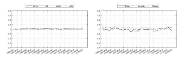
Table 5 shows the mean value of dynamic correlation sequence between the oil-specific demand shock and the macroeconomic variable we obtain empirically. Figures 1215 show that the dependence between the oil-specific demand shock and macroeconomic variables of oil import and export countries exhibit obvious dynamics.
Table 5 Mean value of dynamic correlation sequence between the oil-specific demand shock and the macroeconomic variables |
| | Importer | | Exporter |
| China | U.S. | Japan | India | Brazil | Canada | Russia |
| IOI | 0.23 | 0.20 | 0.30 | 0.16 | | 0.21 | 0.40 | 0.16 |
| EPU | 0.24 | 0.26 | 0.03 | 0.04 | 0.39 | 0.39 | 0.45 |
| CPI | 0.08 | 0.29 | 0.77 | 0.02 | 0.07 | 0.45 | 0.01 |
| EXR | 0.14 | 0.01 | 0.00 | 0.03 | 0.02 | 0.13 | 0.01 |
Figure 12 Dynamic dependence between oil-specific demand shock and IOI of importers and exporters |
Full size|PPT slide
Figure 13 Dynamic dependence between oil-specific demand shock and EPU of importers and exporters |
Full size|PPT slide
Figure 14 Dynamic dependence between oil-specific demand shock and CPI of importers and exporters |
Full size|PPT slide
Figure 15 Dynamic dependence between oil-specific demand shock and EXR of importers and exporters |
Full size|PPT slide
As for the industrial output, Table 5 shows that the impact of the oil-specific demand shock on the industrial output of oil importing countries is negative and that of oil exporting countries is positive except for Brazil. Intuitively, the rise of the oil price, raises the oil acquisition costs of importing countries and affects adversely their industrial production, and increases the profitability of exporting countries driving indirectly domestic economic development and has a positive effect on their industrial output. From Figure 12 we can find that the positive correlations of Canada and Russia have a sudden decline after 2008 while the negative correlations of four importing countries become weakened (the weakening of China is lagged) in virtue of the speculation inhibited by the financial crisis. In addition, the negative correlation of India decreases close to zero in 2011, probably on account of the oil supply shock is the main effect during this period. From 2013 to 2015, the negative correlation of Japan is strong indicating the large impact of oil-specific demand shock on the industrial output.
As for the economic policy uncertainty, as can be seen from Table 5, as a whole, all exporting countries shows a significantly negative correlation. It is well understood that the high oil price and the shortage of future oil supply are undoubtedly good news for exporters with large reserves of petroleum resources, which benefits their economic stability. On the contrary, the United States shows a significantly positive correlation, which is well understood as an oil importing country. China's negative correlation may be due to the Chinese government's control over the market because, as mentioned earlier, China is a very policy-oriented market. The Chinese government will control the domestic oil price under the oil-specific demand shock from the international market ensuring domestic economic policy stable. As for Japan and India, the almost irrelevance shows that the economic policy uncertainty of these two countries is extraneous with the oil-specific demand shock. From Figure 13, the exporting countries show strong negative correlations during the period after the financial crisis in 2008, which shows that the crisis of the oil-specific demand shock at this time can reduce the economic policy uncertainty. As indicated earlier, any rise in oil prices could bring crisis to a halt in a crisis of falling oil prices, especially for exporting countries, with favorable economic recovery.
As for the inflation, as a whole, the dependence between the oil-specific demand shock and the inflation of importing countries is negative and that of exporting countries is positive expect for Russia as shown in Table 5. This shows that when the oil-specific demand shocks occur, the inflation in importing countries decreases and the inflation in exporting countries rises. The rising inflation in the exporting countries is understandable because the exporting countries selected in this paper are not based on the petroleum exploitation industry as the main economic pillar and the rise of oil prices will raise the production costs of various industries in these exporting countries pushing up the price level. However, the reduction of the inflation in importing countries is totally contrary to logic. Generally speaking, the soaring of the international oil price raises the import cost of importing countries resulting in the import-oriented inflation. This is difficult to get a reasonable explanation. In this paper, we provide a possible way of thinking, that is, in response to the exporting country's control over the pricing right of oil, importing countries have established oil reserve systems and actively developed offshore oil extraction technologies to deal with the import-oriented inflation.
As for the real exchange rate, as shown in Table 5, the correlation between the oil-specific demand shock and the real exchange rate of these countries is weak and the exchange rates of China and Canada are affected harder by the negative oil-specific demand shock, relatively speaking, resulting in the domestic currency devaluation. As can be seen from Figure 15, the correlations of China and India reaches a negative minimum at the financial crisis in 2008, indicating that during this period, the oil-specific demand shocks have caused the real effective exchange rate index of the two countries to decline and the foreign currency devaluation. After 2011, the intensity of negative correlation in China weakened, and the effect of the oil-specific demand shocks decreased. In India, the correlation turns from negative to positive, that is, the the oil-specific demand shock during this period raises the real effective exchange rate index rise and currency appreciation.
4.3 The Dynamic Impact of Structural Oil Prices Shocks on Macro-Economy
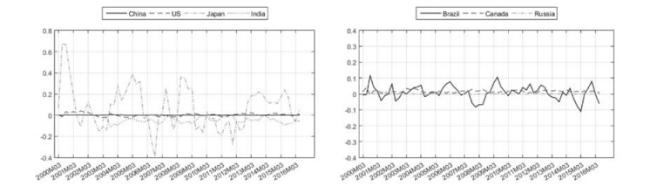
From the empirical results above, we have found there do exist impacts of oil price shocks on the macroeconomic variables and the dependence between them exhibit dynamic characteristics. After that, we apply the measure, ΔCoE, proposed in Subsection 2.3 to quantify the impact intensity conditional on the for the oil shock at the 90% confidence level ().
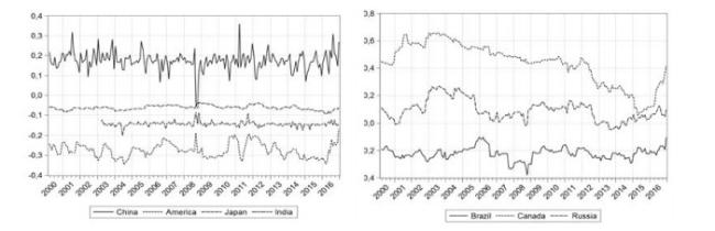
As for the impact of oil supply shocks, we can find that the impact of oil supply shocks on the macroeconomic variables exhibit dynamic characteristics for different countries and different periods with different degrees as shown in Figures 1619. From these figures, we can find that the impacts of oil supply shocks on the industrial output and exchange rates is weak and the changes are less than 10 percent. For the inflation, oil supply shocks show a very strong effect on Japan's domestic price level in different times, for instance, the increase level reached 40% during global financial crisis and drop down after the crisis as shown in Figure 18. The impact on Brazil's inflation is a little stronger than other oil exporting countries but still weak, around 10 percent. In addition, the effect of oil supply shocks on economic policy uncertainty is found more strong than other variables excluding for Japan. For example, the impact for China shows significant rise positively during crisis and declines down to negative as shown in Figure 19. Three oil exporting countries show more stronger response to oil supply shocks than oil importing countries.
Figure 16 Dynamic impacts of oil supply shocks on IOI of importers and exporters |
Full size|PPT slide
Figure 17 Dynamic impacts of oil supply shocks on EXR of importers and exporters |
Full size|PPT slide
Figure 18 Dynamic impacts of oil supply shocks on CPI of importers and exporters |
Full size|PPT slide
Figure 19 Dynamic impacts of oil supply shocks on EPU of importers and exporters |
Full size|PPT slide
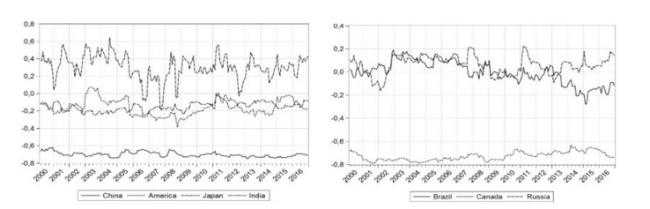
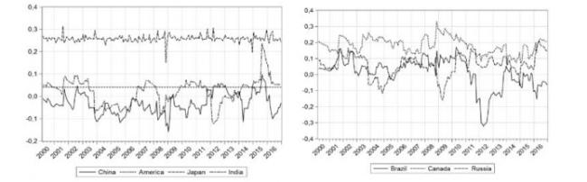
As for the impact of aggregate demand shocks, from Figure 20, we can find that the dynamic effect of the aggregate demand shock on the industrial output of both oil importing countries and oil exporting countries are positive but most are less than 10%, which is similar to the results obtained from the previous sections, and also show time-variation. The impact of this kind of shock on exchange rate is weak for countries because of the economic prosperity. In addition, the aggregate demand shock on the inflation of India and America is stronger than other countries, such as, rising 20% for India, and the impact for Brazil is negative all the time. Figure 23 shows that the economic policy uncertainty can be affected by aggregate demand shocks more than other variables. The impact intensity can reach up to 30% during crisis and drop down to 50% before and after the crisis. The effect for China and India is stronger than US and Japan, and effects for Canada and Russia is stronger than Brazil. Interestingly, the impact on economic policy uncertainty for China and India is opposite and that for Canada and Russia is identical broadly.
Figure 20 Dynamic impacts of aggregate demand shocks on IOI of importers and exporters |
Full size|PPT slide
Figure 21 Dynamic impacts of aggregate demand shocks on EXR of importers and exporters |
Full size|PPT slide
Figure 22 Dynamic impacts of aggregate demand shocks on CPI of importers and exporters |
Full size|PPT slide
Figure 23 Dynamic impacts of aggregate demand shocks on EPU of importers and exporters |
Full size|PPT slide
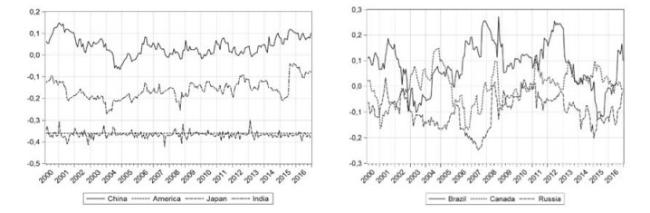
As for the impact of oil specific shocks, we find that the dynamic impact of oil-specific demand shocks on the macroeconomic variables of each country is shown in Figures 2427. From Figure 24, we can find that China and India's industrial output are affected by oil-specific demand shocks more strongly than U.S. and Japan, and also show the opposite direction as same as the impact of aggregate demand oil shocks on their economic policy uncertainty. Basically, the impact of this shock on oil exporting countries is positive and weak. As for the exchange rates, the impact for China and Japan is negative and that for America is positive in oil importing countries. For oil exporting countries, the impact is basically positive as shown in Figure 25. We also find that the effect of oil-specific demand shocks on the inflation is stronger for India than other oil importing countries. For oil exporting countries, Canada's inflation is affected positively all the time and Brazil's inflation is affected negatively in most periods, particularly in financial crisis. From Figure 27, we can find oil-specific demand shocks can also affect economic policy uncertainty more strongly than other variables for both oil importing and exporting countries. These effects are positively significant for oil importing countries during crisis period, such as India's 40% rising, and negatively significant for oil exporting countries in most time, such as Canada's 20% dropping.
Figure 24 Dynamic impacts of oil-specific demand shocks on IOI of importers and exporters |
Full size|PPT slide
Figure 25 Dynamic impacts of oil-specific demand shocks on EXR of importers and exporters |
Full size|PPT slide
Figure 26 Dynamic impacts of oil-specific demand shocks on CPI of importers and exporters |
Full size|PPT slide
Figure 27 Dynamic impacts of oil-specific demand shocks on EPU of importers and exporters |
Full size|PPT slide
5 Conclusions
In this paper, we apply the international oil market SVAR model proposed by Kilian
[16] to decompose the international oil prices shock into the oil supply shocks, the global aggregate demand shocks and the oil-specific demand shocks. Then, we use the DCC-GARCH model to study the dynamic dependence between three oil price shocks and macroeconomic variables of the selected countries. In addition, we propose the conditional expectation (CoE) to quantify the intensity of the impact of the oil price shock on the macroeconomic variables. We employ the time-varying copula to calculate the CoE for different time. We take the major oil importing and exporting countries in the world (importers: China, U.S., Japan and India, exporters: Brazil, Canada and Russia) into consideration. From the perspective of oil importing and exporting, we discuss the commonalities and differences in the impact of the oil shocks on macro-economy of different countries. Furthermore, we also consider various macroeconomic variables (industrial output, economic policy uncertainty, inflation, exchange rate) and discuss the macroeconomic impact of oil shocks on an economy from a more complete perspective.
Through empirical research, we obtain three main conclusions as follows: Firstly, the impact of these three oil price shocks on macroeconomic variables does have time-varying characteristics and the degree and direction of this impact are different in different periods. However, there are still some impacts keeping positive or negative all the time, such as the negative impact of oil-specific shocks on Canada's economic policy uncertainty. Secondly, for different countries, the impact of oil shocks on macroeconomic variables is also different as expected. Additionally, there exist some interesting results: For oil importing countries, the oil supply shock is not conducive to the stability of economic policies and the oil-specific demand shock has a negative impact on industrial output; for oil exporting countries, the oil-specific demand shock has a positive impact on the industrial production and a negative impact on the economic policy uncertainty; for oil importers and exporters, the oil supply shock will aggravate inflation and the global aggregate demand shock is conducive to the stability of economic policy. The aggregate demand shock and oil-specific shock affect the emerging countries (e.g., China and India) more strongly than developed countries (e.g., U.S. and Japan). Moreover, the impact of oil shocks on economic policy uncertainty is more significant than other macroeconomic indicators. Thirdly, the empirical results show the evidence that most of correlations between oil shocks and the macroeconomic variables are weak while some of correlations are strong and represent national characteristics. For instance, the dependence between oil supply shocks and India's industrial output is significantly negative as well as the inflation of China and Canada. There exists a significantly positive correlation between global aggregate demand shocks and China economic policy uncertainty.
Furthermore, we propose some suggestions based on empirical results: Firstly, there exist the significantly disadvantageous effects of the oil supply shock on oil importing countries and they should be prudent, and through the establishment and improvement of the strategic petroleum reserve system, by strengthening the research of offshore oil exploration and mining technology and developing the new energy to replace oil, increase oil reserves to weaken the effect of oil supply shocks. Secondly, the oil-specific demand shock is conducive to the industrial production and the stability of economic policy of oil exporting countries, and the exporters can seize the opportunity to develop their own economy. Thirdly, oil supply shocks could exacerbate inflation for both oil importers and exporters, so the government should be alert to the international oil supply shock. Oil exporting countries should take the adverse effects of the oil cut on their own price level into consideration when they establish the oil production strategy. Meanwhile, oil importing countries should develop the price stabilization policy to copy with the possible oil supply shocks and finally solve the oil problem through the technological innovation and the development of new sustainable energy sources.
Finally, we also give some suggestions as there exist some special results for China including the significantly negative correlation between oil supply shocks and China inflation, the significantly positive correlation between global aggregate demand shocks and the economic policy uncertainty of China and the negative correlation between oil-specific demand shocks and China economic policy uncertainty. On the one hand, the government of China should be highly vigilant about the import-oriented inflation caused by oil supply shocks and the specific measures should be the same as that of oil importing countries. On the other hand, the Chinese government should appropriately control the oil market for the reason that controlling oil price is not conductive to the stability in economic prosperity while the oil controlled policy have a advantage of the politic stability when the oil price is falsely high or the expectation of the further oil price rises. Then, how to make the reasonable dynamic policy to control the oil price could be a meaningful problem.
{{custom_sec.title}}
{{custom_sec.title}}
{{custom_sec.content}}
 PDF(1247 KB)

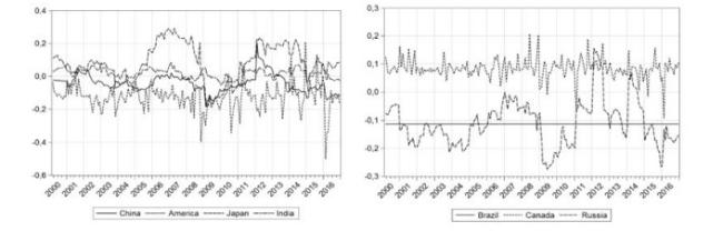
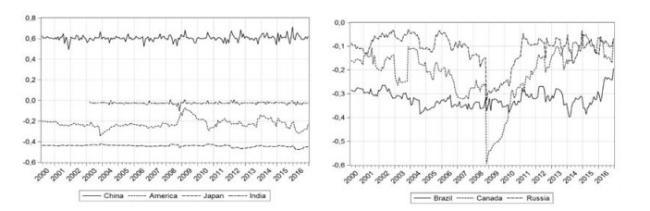
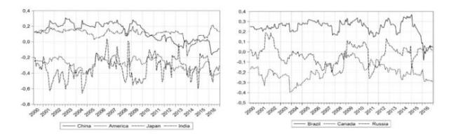
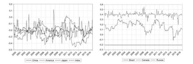
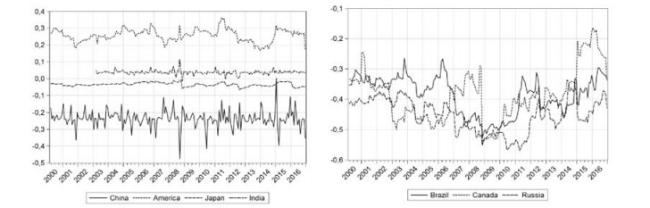
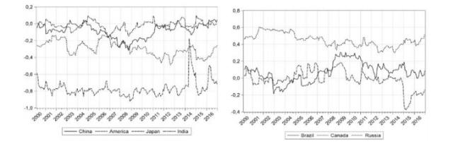
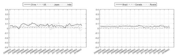
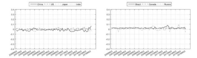
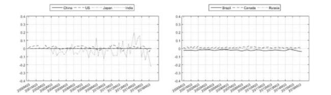
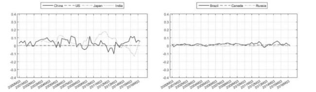
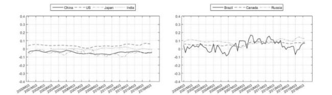
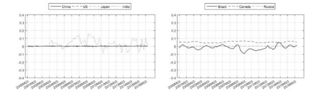
 Table 1 Descriptive statistics of the sample series
 Figure 1 Response of industrial output, exchange rates, inflation, and economic policy uncertainty to oil supply shocks


