The Effect of Green Technology Adoption Strategy on Duopoly Competition

Chenglin SHEN; Xinxin ZHANG

doi:10.21078/JSSI-2021-498-21

PDF(310 KB)

Journal of Systems Science and Information ›› 2021, Vol. 9 ›› Issue (5) : 498-518. DOI: 10.21078/JSSI-2021-498-21

The Effect of Green Technology Adoption Strategy on Duopoly Competition

Author information +

History +

Abstract

Given consumers' trade-offs between conventional economic and environmental attributes of products, we provide a game-theoretic model to explore the role of GTA strategy in duopoly competition by incorporating two salient features: Two product types-The green product produced by a firm with GTA strategy and the ordinary product produced by a firm without GTA strategy, and two consumer segments, i.e., the green consumers who are willing to pay for green products and the ordinary consumers who are willing to pay for ordinary products. Our analysis shows that GTA strategy may either increase or decrease the green firm's quality provision. The subtle relationship between the green firm's quality strategy and GTA strategy not only affects its own equilibrium performances but its rival's. We also find that two consumer segments may be better off in the presence of a lower GTA intensity. Additionally, although the GTA strategy benefits the environment, the GTA investment is not the more the better. Finally, we find that GTA strategy would lead to higher social welfare only when the GTA efficiency is high enough. Our work not only provides an alternative economic explanation why some firms choose to implement GTA strategy and some do not in reality, but gives managerial insights for firms with different GTA strategies as well as policy insights for the social planner.

Key words

green technology adoption (GTA) / duopoly competition / quality provision / game theory

Cite this article

EndNote

Ris (Procite)

Bibtex

Download Citations

Chenglin SHEN , Xinxin ZHANG. The Effect of Green Technology Adoption Strategy on Duopoly Competition. Journal of Systems Science and Information, 2021, 9(5): 498-518 https://doi.org/10.21078/JSSI-2021-498-21

1 Introduction

Increasing social concerns over environmental deterioration and consequences push manufacturers to reconsider their current production practice and look for ways to mitigate environmental damages. One of efficient solutions to deal with this problem is to adopt green technology^[1]. As a result, many manufacturers, such as Toyota, Haier, etc., have invested in green technology adoption strategy (GTA strategy, for short) and started to provide green products and solutions^[2]. Another key driver for the success of GTA strategy is the emergence of green consumerism. It is worth mentioning that as "green" penetrates everyday life, a growing number of consumers place significant importance on eco-friendly consuming and even are willingness to pay a premium for the green product. According to Du, et al.^[3], Tully and Winer^[4], upwards of 60% of respondents are willingness to pay 16.8% premium on average for eco-labeled products.

Although GTA strategy is empirically proved to have a positive effect on firms' economic and environmental performance^[5-7], quite a few of manufacturers do not implement green production option in reality. Such a phenomenon is explained mainly from the trade-off between benefits and costs associated with GTA strategy: GTA strategy requires substantial up-front capital investments, and frequently resulting in an increase in total production cost as well. Higher implementing cost on GTA strategy might keep manufacturers away from this kind of strategy^[8]. At the same time, it is noteworthy that not all customers would tend to purchase green products. Contingent on product categories, only 15%

\sim

46% of the overall customer market would be inclined to choose green products^[9]. In particular, rational consumers usually need to balance the trade-off between conventional economic attributes of a product such as price and quality, etc. and environmentally friendly features, and then make purchasing decisions^[10]. It is clear that the GTA strategy would have a direct impact on both the profitability of firms and the purchasing behavior of consumers. What is less clear, however, is how the GTA strategy—be it a result of environmental consciousness, economic opportunities, or both—impacts firms' incentives for quality provision in a duopoly market consisting of firms with and without GTA strategy. Given the scarcity of economic resources, firms in reality usually encounter how to coordinate the GTA strategy and a firm's quality strategy. In other words, a firm's GTA choice is usually intertwined with its quality provision which in turn influences pricing decisions, demands and profits of both the manufacturer itself and its rival as well as consumer surplus and social welfare.

To better understand how firms with different GTA strategies should choose their product quality and price levels and how the GTA strategy influences firms' profits, consumer surplus as well as social welfare, we design a competition model between firms with different GTA strategies to investigate firms' pricing and quality decisions. In particular, we attempt to provide insights to the following research questions: What quality and price levels should the firms with different GTA strategy provide in duopoly competition? Considering consumers' premium for the green product, does the firm with GTA strategy necessarily earn profitable advantages compared with its ordinary rival? If no, on what condition could the firm with GTA strategy achieve competitive advantages in terms of gaining profits? How are consumer surplus, the environment and social welfare affected by the GTA strategy?

This paper uncovers several insights. First, we illustrate how different types of firms in terms of GTA strategy should strategically adjust their optimal quality and pricing decisions according to the dynamics of the GTA intensity and the degree of horizontal differentiation between two competing firms. We also find that the GTA strategy may either enhance or hurt the profit of the firm with GTA strategy, which depends on its GTA efficiency and the degree of horizontal differentiation between the firm and its rival. We further conduct the welfare analysis to investigate the interplay of the GTA investment intensity and the competition intensity (measured by the degree of horizontal differentiation between two competing firms), and find that consumers might be either better off or worse off in the wake of GTA strategy. Meanwhile, the GTA strategy does not necessarily improve social welfare. Only when the GTA efficiency is fairly high, could social welfare be enhanced. In summary, our results not only make guidelines for business managers to conduct optimal competitive strategies and make proper decisions on their quality provisions and prices, but also guide social planners to make policies to promote GTA and mitigate environmental damages.

The rest of the paper is organized as follows. The following section reviews the related literature. Section 3 models the competition between the firm with GTA strategy and the one without GTA strategy. Section 4 characterizes two firms' equilibrium decisions and reveals the influences of GTA strategy on firms' equilibrium decisions as well as on their profits. Section 5 conducts welfare analysis, and analyzes effects of the GTA strategy on consumer surplus, environment and social welfare. Finally, section 6 concludes with a discussion of the main themes and managerial insights of the paper and provides directions for future research. All proofs are provided in Appendix A

\sim

2 Literature Review

Our work is primarily related to two literature streams: The literature on sustainable operations with green technology adoption in a competitive market and the literature on product quality choice. In what follows, we briefly review literature and point out our contribution relative to these works.

With the successful adoption of green technology in many industries, a growing amount of papers pay serious attention to the competitive strategy of green manufacturers. However, most studies in this field consider a symmetric competitive setting in which several competing manufacturers have the same capacities to provide green products. In these papers (see [11-15] for examples), manufacturers usually first decide on the level of greenness of their products and then engage in price/quantity competition. To our best knowledge, there are only a few of papers involving an asymmetric competition between firms with and without green production (e.g., the brown manufacturer and the green one). Galbreth and Ghosh^[16] incorporates sustainable concern and awareness into a model of horizontal competition in a duopoly and investigates the impacts of consumer's awareness on both high sustainable and low sustainable firms. Zhou^[17] considers a duopoly completion between a brown firm and a green one in the presence of green consumers who are willing to pay a price premium for the green product and discuss the optimal pricing decisions of both types of firms. Our work makes a substantive contribution to this stream by incorporating the quality choices of firms with and without GTA strategy in addition to pricing decisions. More importantly, we demonstrate that with GTA strategy one firm can either increase or decrease in its quality provisions depending on the degree of horizontal differentiation between two competing firms, which further influence two firms' profits, consumer surplus of the green segment and the ordinary segment as well as social welfare.

There have been numerous works on product quality choices in both the marketing and operations management literature. Included in this stream is the literature on market segmentation and product differentiation^[18-20]. Much of this stream of literature focuses on the optimal quality and pricing decisions of a product line that is differentiated by quality in the context of different types of consumer heterogeneities in their willingness to pay. Among this stream of literature, [10] is particularly instrumental to our work because it provided the inspiration and basis for both quality choices and the notion that green consumers are willing to pay a price premium for eco-friendly product everything else being equal that we adopt, but our work differs from theirs in three important respects. First, we use a competitive game model to capture the quality-price competition between firms with and without GTA strategy while Gu, et al.^[10] only considers monopolist's quality choices and pricing decisions in the context of remanufacturing. Second, we incorporate both vertical and horizontal differentiation between two types of firms. The combination of horizontal and vertical differentiation not only captures the reality better but also provides additional insights that could be overlooked in one-dimensional differentiation model (e.g., horizontal differentiation or vertical differentiation)^[21]. Third, we conduct welfare analysis to reveal how the GTA strategy implemented by one firm affects different consumer segments as well as social welfare, which provides policy insights for social planner to induce manufacturers to optimize their green technology adoption for enhancing the allocation efficiency of the market.

3 Model Descriptions and Notations

We develop a stylized game theoretical model to examine the quality-price competition between two firms with different GTA strategy, i.e., only one firm can make green technology investment but the other firm cannot. This corresponds to the reality that green technology adoption is unbalance across the whole industry, e.g., only some firms have mastered green technologies or have enough money to adopt green technologies. The similar scenario is considered in Zhou^[17] and Ma, et al.^[22]. For ease of exposition, we refer to the firm with GTA strategy as the green firm (i.e., Firm

G

, for short) and refer to the firm without GTA strategy as the ordinary firm (i.e., Firm

O

, for short). Although the green product and the ordinary product are distinct in both quality (vertical differentiation) and category (horizontal differentiation), they are assumed to be functionally substitutable. To maximize their respective profits, two types of firms decide optimal quality and price levels to compete.

Following Du, et al.^[3], we assume that the green product is different from the ordinary one on both consumer's willingness-to-pay and total production cost. With the growing trend of green consumerism, consumers value more about green products than its ordinary counterparts, in spite of two types of products with similar functionality. To model this, we introduce a term of consumer's premium for green products,

β \in (0, 1]

to denote the additional utility from purchasing a green product. In other words, consumers' valuation for the green product is (

1 + β

) times of their willingness-to-pay for the ordinary product. The assumption is common in the green production and marketing literature (see [3], [10], and [17] for example). Generally speaking, the more a firm invests in GTA strategy, the greener products are offered, which in turn leads to a higher additional utility for consumers. Hence, from firm perspectives, parameter

β

can also be viewed as a firm's GTA intensity reflecting the firm's effort/investment in GTA strategy. Note that if

β = 0

, then there are no green products offered because no firm implements GTA strategy.

On the other hand, to implement green technology, a firm needs to invest in green technology development. In particular, we model the investment cost as a quadratic function,

η β^{2}

, increasing with the GTA intensity

β

, where

η

is the unit cost on GTA strategy capturing the efficiency of a firm to successfully implement green technology. To ensure the existence of the optimal GTA investment in equilibrium and avoid triviality, we assume that

η > \frac{(18 k t - 1) k v^{2}}{4 {(9 k t - 1)}^{2}}

, which implies the green firm's profit function is single-peaked, quadratic functions in terms of GTA investments. This technical condition also guarantees that the green firm has an incentive to adopt green technology. For convenience, we use the subscript "

g

" to express the green firm and green products and "

o

" to express the ordinary firm and ordinary products respectively in the rest of the paper.

The product market consists of a continuum of consumers with its size normalized to one uniformly distributed on the interval

[0, 1]

. Each consumer considers green product, ordinary product, as well as no purchase options and purchases at most one to maximize her utility. Given that consumers might be loyalty to the firm, or preference for a brand in reality, we assume that consumers have heterogeneous preferences between firms. We adopt a stylized Hotelling model to capture consumers' various tastes^[23], where consumers are assumed to be uniformly distributed along a unit line in the preference space with Firm

G

located at 0 and Firm

O

located at 1. The consumer's disutility from non-exactly matched preference is

t d_{i}

, where

d_{i}

is the distance between consumer's location

x

and product i's location;

t

(

t > 0

) is the unit cost of misfit (traditionally called consumer's misfit cost or transportation cost) capturing consumer's preferences for product fit which can also be interpreted as reflecting the degree of horizontal differentiation between two firms. By definition, it is straightforward to derive that

d_{i} = x

for

i = g

and

d_{i} = 1 - x

for

i = o

. In summary, consumer's location

x \in [0, 1]

in the unit line represents the consumer's preference toward a product.

Next, we elaborate on two firms' demand functions based on the utilities of consumers. Given firms' quality levels (

s_{i}

) and prices (

p_{i}

), a consumer located at

x

obtains a net utility of

U_{o} = v + s_{o} - t (1 - x) - p_{o}

when purchasing an ordinary product and

U_{g} = (1 + β) v + s_{g} - t x - p_{g}

when purchasing a green product, where

v

is the reservation utility for products. We further assume that

v

is sufficiently large so that the market is fully covered. Without loss of generality, we assume that consumers' outside option has a utility of zero; consumers will thus buy the product that yields a higher non-negative utility.

By solving

U_{g} = U_{o}

, we derive the marginal location

\hat{x} = \frac{1}{2} + \frac{β v + s_{g} - s_{o} - p_{g} + p_{o}}{2 t}

, where a consumer is indifferent between the two types of firms. The marginal location divides the market into two parts, and each part represents the market share from one firm. Firm

G

's market share is composed of consumers whose utility

U_{g}

is higher than

U_{o}

, and vice versa. To maximize consumers' utilities, we derive the demand functions of Firm

G

and Firm

O

, respectively.

\begin{array}{rcl} q_{g} (p_{g}, p_{o}, s_{g}, s_{o}) = {\begin{cases} 0, & i f β v \leq p_{g} - p_{o} - t - s_{g} + s_{o}, \\ \hat{x}, & i f p_{g} - p_{o} - t - s_{g} + s_{o} < β v \leq p_{g} - p_{o} + t - s_{g} + s_{o}, \\ 1, & i f β v > p_{g} - p_{o} + t - s_{g} + s_{o}, \end{cases} \end{array}

(1)

\begin{array}{rcl} q_{o} (p_{g}, p_{o}, s_{g}, s_{o}) = {\begin{cases} 1, & i f β v \leq p_{g} - p_{o} - t - s_{g} + s_{o}, \\ 1 - \hat{x}, & i f p_{g} - p_{o} - t - s_{g} + s_{o} < β v \leq p_{g} - p_{o} + t - s_{g} + s_{o}, \\ 0, & i f β v > p_{g} - p_{o} + t - s_{g} + s_{o} . \end{cases} \end{array}

(2)

As shown in (1) and (2), only when the additional valuation

β v

is in the middle range (i.e.,

p_{g} - p_{o} - t - s_{g} + s_{o} < β v \leq p_{g} - p_{o} + t - s_{g} + s_{o}

), both firms can achieve positive market shares. Otherwise, Firm

G

(Firm

O

) will be squeezed out of market if

β v

is very large (small).

In order to characterize profit functions, we assume that the two firms have a similar cost structure including a marginal production cost and an additional cost associated with the quality level of a product,

s_{i}

. Consistent with previous literature of quality and price competition (see [24-26] for example), each firm is assumed to incur a constant unit production cost

c

and an increasing quadratic quality cost

k s_{i}^{2}

, independent of the production volume, where

k

is the unit cost of quality. Firm

G

also burdens GTA cost in addition to the marginal production cost and quality cost. In summary, the profit functions of Firm

G

and Firm

O

can be expressed as

\begin{array}{rcl} \begin{array}{rcl} Π_{g} (p_{g}, s_{g}) = (p_{g} - c) q_{g} - k s_{g}^{2} - η β^{2}, \end{array} \end{array}

(3)

\begin{array}{rcl} \begin{array}{rcl} Π_{o} (p_{o}, s_{o}) = (p_{o} - c) q_{o} - k s_{o}^{2} . \end{array} \end{array}

(4)

We develop a two-stage game model to reveal optimal strategies for the duopoly competition. The timing of the game is as follows. In the first stage, Firm

G

and Firm

O

simultaneously choose their respective product quality levels

s_{i}

. In the second stage, both firms announce prices

p_{i}

simultaneously to compete based on their first-stage quality choices. After observing

s_{i}

and

p_{i}

, consumers decide which firm to visit. All notations used in this paper are summarized in Table 1.

Table 1 Notations for variables and parameters

Notations	Description
$p_{g}$	Price of green products
$p_{o}$	Price of ordinary products
$s_{g}$	Quality level of green products
$s_{o}$	Quality level of ordinary products
$q_{g}$	Sales of green products
$q_{o}$	Sales of ordinary products
$β$	GTA intensity
$v$	Consumer's reservation valuation for a unit product
$c$	Marginal production cost
$k$	Unit cost of quality
$η$	Unit cost of GTA strategy
$t$	Consumer's misfit cost
$x$	Location of the consumer in the unit Hotelling line
$e_{g}$	Emission per unit green product
$e_{o}$	Emission per unit ordinary product
$Π_{g}$	Profits of Firm $G$
$Π_{o}$	Profits of Firm $O$
$I_{g}$	Environmental impact of green production
$I_{o}$	Environmental impact of ordinary production
CS	Consumer's surplus
SW	The social welfare

4 Equilibrium Analysis

In this section, we first characterize the equilibrium outcome of the two-stage competitive game, and then obtain conditions under which the GTA strategy is beneficial to Firm

G

by comparing equilibrium outcome of its rival (i.e., Firm

O

). As is common practice, we use backward induction to analyze pricing decisions in the second stage. Given

s_{g}

and

s_{o}

offered in the first stage, solving the maximization problems for two firms derives the optimal prices of two firms as follows.

\begin{array}{rcl} {p_{g}}^{*} (s_{g}, s_{o}) = t + c + \frac{β v + s_{g} - s_{o}}{3}, \end{array}

(5)

\begin{array}{rcl} {p_{o}}^{*} (s_{g}, s_{o}) = t + c - \frac{β v + s_{g} - s_{o}}{3} . \end{array}

(6)

We now digress to discuss our implicit assumption of a competitive (rather than a monopoly) equilibrium in which both firms have positive market shares. For any firm i to profitably sell its product, its price must cover its marginal cost, that is,

{p_{i}}^{*} (s_{g}, s_{o}) > c

, where

i = g, o

; otherwise, the firm will prefer not selling and have a zero sales. The necessary condition for a competitive pricing equilibrium straightforwardly simplifies to

| β v + s_{g} - s_{o} | < 3 t

. Note that

(1 + β) v + s_{g} - c

(

v + s_{o} - c

) is the marginal cost of Firm

G

(Firm

O

) the highest willing-to-pay consumer's valuation subtracted by the marginal cost of Firm

G

(Firm

O

) and that this essentially represent how competitive Firm

G

(Firm

O

) can be. Thus, the condition,

| β v + s_{g} - s_{o} | < 3 t

, is quite intuitive; it simply states that the difference in firms' feasible profit margins must be lower than a certain threshold; otherwise, there may not be a pure-strategy pricing equilibrium, or the more efficient firm will squeeze the other out of the market and become a monopoly.

Substituting (5) and (6) into (3) and (4), we simplify the firms' profits to

\begin{array}{rcl} \begin{array}{rcl} Π_{g}^{*} (s_{g}, s_{o}) = \frac{{(β v + s_{g} - s_{o} + 3 t)}^{2}}{18 t} - k s_{g}^{2} - η β^{2}, \end{array} \end{array}

(7)

\begin{array}{rcl} \begin{array}{rcl} Π_{o}^{*} (s_{g}, s_{o}) = \frac{{(β v + s_{g} - s_{o} - 3 t)}^{2}}{18 t} - k s_{o}^{2}, \end{array} \end{array}

(8)

where the sales of Firm

G

and Firm

O

are given by

q_{g} = \hat{x} = \frac{β v + s_{g} - s_{o} + 3 t}{6 t}

and

q_{o} = 1 - \hat{x} = \frac{- β v - s_{g} + s_{o} + 3 t}{6 t}

, respectively.

We now solve the first-stage game. In the first stage, two types of firms simultaneously choose their quality levels to maximize respective profits shown in (7) and (8). Additionally, to guarantee the existence of a competitive equilibrium, the degree of horizontal differentiation between two firms cannot be too small. In other words, parameter

t

should be larger than a certain threshold. In particular, we assume that

t > \frac{1}{18 k}

, which implies that both firms' profits are single-peaked, quadratic functions in terms of their quality levels. By solving

\frac{\partial Π_{g}^{*} (s_{g}, s_{o})}{\partial s_{g}} = 0

and

\frac{\partial Π_{o}^{*} (s_{g}, s_{o})}{\partial s_{o}} = 0

simultaneously, we derive Proposition 1 which summarizes the equilibrium decisions of duopoly firms.

Proposition 1 There exists a unique pure-strategy sub-game perfect Nash equilibrium $($ SPNE $)$ under conditions of $β < \frac{| 9 k t - 1 |}{3 k v}$ and $t > \frac{1}{18 k}$ . The SPNE is given by $s_{g}^{*} = \frac{1}{6 k} + \frac{β v}{2 (9 k t - 1)}$ , $s_{o}^{*} = \frac{1}{6 k} - \frac{β v}{2 (9 k t - 1)}$ ; ${p_{g}}^{*} = t + c + \frac{3 k t β v}{9 k t - 1}$ , ${p_{o}}^{*} = t + c - \frac{3 k t β v}{9 k t - 1}$ ; ${q_{g}}^{*} = \frac{1}{2} + \frac{3 k β v}{2 (9 k t - 1)}$ , ${q_{o}}^{*} = \frac{1}{2} - \frac{3 k β v}{2 (9 k t - 1)}$ .

Proposition 1 provides two conditions that are needed for the existence of competitive equilibrium. First, the degree of horizontal differentiation between two firms cannot be too small (i.e.,

t > \frac{1}{18 k}

), which ensures the existence of optimal quality levels for both firms. The second condition requires that the green firm's GTA strategy is not too "effective" at increasing consumers' valuations for green products, that is, the GTA intensity cannot be too large (i.e.,

β < \frac{| 9 k t - 1 |}{3 k v}

). Otherwise, the efficient firm will be able to profitably squeeze out its competitor and become a monopoly firm.

Proposition 1 also shows that Firm

G

does not necessarily achieve higher quality and price levels as well as the resulted sales than does its ordinary counterpart (i.e., Firm

O

) in equilibrium. When the degree of horizontal differentiation between two firms is large enough (i.e.,

t > \frac{1}{9 k}

), the GTA intensity always leads to increase in the green firm's optimal quality level, price and the resulted sales and decrease in the ordinary firm's optimal quality level, price and the resulted sales, and vice versa. Therefore, we naturally put forward a question: How does the GTA intensity (

β

) influence two types of firms' equilibrium outcome? In other words, does the GTA strategy necessarily increase Firm

G

's optimal quality level, price and the resulted sales? To answer this question, it is necessary to take the case that no firm implements GTA strategy (i.e.,

β = 0

) into account as a benchmark. We use the superscript

N

to denote the scenario in which on firm chooses GTA strategy. The equilibrium outcome in this case is given by Corollary 1, which is derived directly from Proposition 1.

Corollary 1 When no firm implements the green production $($ i.e., $β = 0)$ , the SPNE is $s_{i}^{N *} = \frac{1}{6 k}$ , ${p_{i}}^{N *} = t + c$ and ${q_{i}}^{N *} = \frac{1}{2}$ . Accordingly, the equilibrium profit is given by $Π_{i}^{N *} = \frac{(18 k t - 1)}{36 k}$ under the condition of $t > \frac{1}{18 k}$ .

When no firm implements GTA strategy, the green firm provides the same equilibrium quality and price levels as its ordinary rival. In addition, two firms split the market and earn same equilibrium profits. By comparing equilibrium outcome with the co-existence of green and ordinary production (shown in Proposition 1), we derive the following corollary.

Corollary 2 In the competitive equilibrium of the co-existence of green and ordinary production:

(i)

t > \frac{1}{9 k}

, a larger

β

will always increase Firm

G

's quality level, price and resulted sales but decrease those of Firm

O

;

(i i)

\frac{1}{18 k} < t < \frac{1}{9 k}

, a higher

β

will increase Firm

O

's outcome but decrease Firm

G

's outcome.

Corollary 2 shows that the GTA strategy may lead to either an increase or a decrease in equilibrium outcome of two firms, which depends on the degree of horizontal differentiation between them. Specifically, if the horizontal differentiation between firms is fairly large (i.e.,

t > \frac{1}{9 k}

), Firm G offers a higher optimal quality level after joining GTA strategy (

s_{g}^{*} > s_{g}^{N *}

). This implies that the GTA strategy and Firm G's quality strategy are complementarity. In such a situation, Firm G's quality level, price and the resulted sales increase with the increase of the GTA intensity. Meanwhile, Firm O has to defensively respond to the GTA strategy (i.e., defensive response) by lowering its own quality and price levels to stay in competition, which may reduce the resulted sales of ordinary products in equilibrium. Otherwise (i.e.,

\frac{1}{18 k} < t < \frac{1}{9 k}

), Firm G offers a lower equilibrium quality level than does in the scenario of no green production (i.e.,

s_{g}^{*} < s_{g}^{N *}

). This implies that the quality strategy and the green firm's GTA strategy are substitutable. In this case, Firm G decreases its quality level, price as well as the resulted sales in equilibrium with the increase of the GTA intensity. Firm O, nevertheless, will aggressively respond to its competitor's GTA strategy by raising quality and price levels as well as the resulted sales.

We have discussed how the GTA intensity affects equilibrium decisions of both firms when the GTA strategy and the green firm's quality strategy are either substitutes or complements. An immediate question arises: Does the GTA strategy always bring competitive advantages for the green firm in terms of gaining profits? To answer the question, we derive the optimal profits of both firms by taking the optimal solutions shown in Proposition 1 back into profit functions shown in (3) and (4).

\begin{array}{rcl} \begin{array}{rcl} Π_{g}^{*} = \frac{(18 k t - 1) {(3 k β v + 9 k t - 1)}^{2}}{36 k {(9 k t - 1)}^{2}} - η β^{2}, \end{array} \end{array}

(9)

\begin{array}{rcl} \begin{array}{rcl} Π_{o}^{*} = \frac{(18 k t - 1) {(- 3 k β v + 9 k t - 1)}^{2}}{36 k {(9 k t - 1)}^{2}} . \end{array} \end{array}

(10)

The next proposition highlights conditions on which the firm with GTA strategy may achieve competitive advantages by using GTA strategy, and how firms' profits affected by the GTA intensity in equilibrium.

Proposition 2 In the competitive equilibrium of the co-existence of green and ordinary production: $(i)$ If $\frac{1}{18 k} < t < \frac{1}{9 k}$ , Firm $G$ always earns a lower profit than Firm $O$ , i.e., $Π_{g}^{*} < Π_{o}^{*}$ . Moreover, a higher $β$ will always increase Firm $O$ 's profit but reduce Firm $G$ 's profit; $(i i)$ If $t > \frac{1}{9 k}$ there exists some $\bar{η} = \frac{(18 k t - 1) v}{3 β (9 k t - 1)}$ such that Firm $G$ is more profitable than Firm $O$ , i.e., $Π_{g}^{*} > Π_{o}^{*}$ , if $η < \bar{η}$ , and vice versa. Moreover, a higher $β$ will always decrease Firm $O$ 's optimal profit but increase Firm $G$ 's optimal profit, if $β < \bar{β} = \frac{(9 k t - 1) (18 k t - 1) v}{3 [4 η {(9 k t - 1)}^{2} - k v^{2} (18 k t - 1)]}$ .

According to Proposition 2, whether Firm G benefits from the GTA strategy critically hinges on the degree of horizontal differentiation between the green firm and its rival. If the degree of differentiation between two firms,

t

is low (i.e.,

\frac{1}{18 k} < t < \frac{1}{9 k}

), Firm G always earns a lower profit than does Firm O in equilibrium. In other words, the GTA strategy will hurt Firm G's profit, indicating that Firm G cannot achieve competitive advantages in terms of gaining profit from the GTA strategy in such a situation. Moreover, a larger GTA intensity (large

β

) will decrease Firm G's optimal profit but increase its rival's optimal profit. This implies that the GTA strategy cannot be an optimal choice for Firm G in such that situation. This occurs because when

t

is low, the GTA strategy and the green firm's quality strategy are substitutes. In such a situation, Firm G's optimal quality level, price and the resulted sales are lower than Firm O, so that Firm G earns a lower profit than its ordinary rival.

By contrast, if

t

is high enough (i.e.,

t > \frac{1}{9 k}

), Firm G might utilize the GTA strategy to reap a higher profit than its ordinary rival only when the GTA efficiency is fairly high (i.e.,

η < \bar{η}

). Note that the GTA intensity might be a double-edged sword for Firm G because the excessive GTA investment will be detrimental to the green firm by lowering its equilibrium profit, although the GTA investment is justified in return on investment (ROI) terms. This outcome stems from two opposing effects of the GTA strategy on Firm G's profitability. First, the GTA strategy plays positive effects on increasing consumers' willingness-to-pay (i.e., {valuation-enhancing effect}), which is beneficial to increase Firm G's profit. Second, a high GTA intensity is also associated with a high GTA cost (i.e, {cost effect}). Depending on which effect dominates, Firm G's profit may increase or decrease as the GTA intensity increases. Particularly, the cost effect dominates when

β > \bar{β}

(i.e., high

β

) whereas the valuation-enhancing effects dominates when

β < \bar{β}

(i.e., small

β

). One managerial implication is that the firm with GTA strategy should optimize its GTA intensity to earn competitive advantage as well as restrict its rival's competitive advantage in terms of gaining profit.

5 Welfare Analysis

In this section, we further investigate the impacts of GTA strategy on consumer surplus (CS) and social welfare (SW). Formally, given consumer's location

x

and price

p_{i}

, the consumer surplus for the firm with GTA strategy (

C S_{g}

) and that for the firm without GTA strategy (

C S_{o}

) are given by

\begin{array}{l} C S_{g} = \int_{0}^{x} [(1 + β) v + s_{g} - t s - p_{g}] d s, \\ C S_{o} = \int_{x}^{1} [v + s_{o} - t (1 - s) - p_{o}] d s . \end{array}

(11)

Substituting results shown in Proposition 1 into (11), the consumer surplus for Firm G and for Firm O in equilibrium are given as follows

\begin{array}{l} {C S}_{g}^{*} = \frac{(3 k β v + 9 k t - 1) [3 k (21 k t - 2) β v + 12 k (9 k t - 1) (v - c) - (9 k t - 1) (15 k t - 2)]}{24 k {(9 k t - 1)}^{2}}, \\ {C S}_{o}^{*} = \frac{(- 3 k β v + 9 k t - 1) [3 k (15 k t - 2) β v + 12 k (9 k t - 1) (v - c) - (9 k t - 1) (15 k t - 2)]}{24 k {(9 k t - 1)}^{2}} . \end{array}

(12)

The effects of GTA intensity on surplus of green consumers and on that of ordinary consumers summarized in the following two propositions.

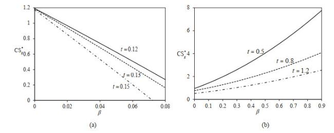
Proposition 3 In competitive equilibrium of co-existence of green and ordinary production: $(i)$ When $\frac{1}{18 k} < t < \frac{1}{9 k}$ , the consumer surplus for Firm G is decreasing in $β$ ; $(i i)$ When $t > \frac{1}{9 k}$ , the consumer surplus for Firm G is increasing in $β$ .

Intuitively, a higher GTA intensity (

β

) is more likely to be beneficial to the green segment because the GTA strategy will bring an additional utility to them. However, we find that this is not necessarily the case. Proposition 3, illustrated in Figure 1, shows that green consumers would be either better off or worse off in the wake of GTA strategy. We observe that a higher GTA intensity might lead to either a decrease or an increase in the surplus of green consumers. The intuition can be explained as follows. When the horizontal differentiation is low, GTA strategy and Firm G's quality strategy are substitutes. In this situation, the stronger the GTA intensity is, the lower quality provision Firm G offers. Thus, the additional utility from GTA strategy does not cover the utility loss resulted from the lower quality levels, which leads to a decrease in the surplus of green consumers. However, when the horizontal differentiation is high, the two kinds of strategy are complements. In such a situation, a higher GTA intensity increases Firm G's quality provision in addition to bring an addition utility to green consumers.

Figure 1 Changes of consumer surplus for the firm without GTA strategy with $β$ under different $t$ ( $v = 3$ , $k = 0.5$ ). (a) when GTA strategy and Firm G's quality strategy are substitutes (i.e., $0.11 < t < 0.22$ ), (b) when GTA strategy and the green firm's quality provision are complements (i.e., $t > 0.22$ )

Full size|PPT slide

From Figure 1(a), we also see that in the case of substitution effect between the GTA strategy and Firm G's quality strategy, as

t

increases, the slope of the curve of green consumer surplus becomes steep implying that a larger horizontal differentiation strengthens the negative effect of GTA intensity on the green consumer. However, according to Figure 1(b), we observe that when the GTA strategy and green firm's quality strategy are complements, as

t

increases, the slope of the curve of green consumer surplus becomes flat, meaning that an increased degree of horizontal differentiation weakens the positive effect of GTA intensity on the green consumer.

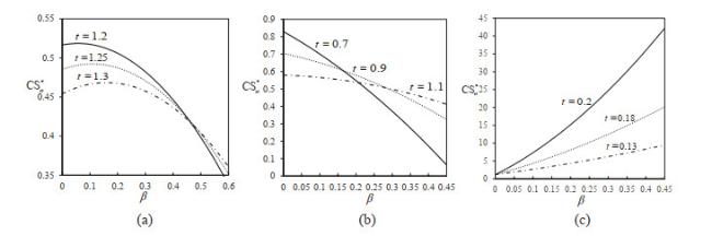
Proposition 4 In the competitive equilibrium of co-existence of green and ordinary production: $(i)$ When $t > \frac{2 + 6 k (v - c)}{15 k}$ holds, there exists some $\hat{β} \in (0, 1)$ such that a larger $β$ will increase the surplus of ordinary consumers, if $β \leq \hat{β}$ , and vice versa; $(i i)$ When $\frac{2 + 6 k (v - c)}{15 k} > t > \frac{1}{9 k}$ holds, a larger $β$ will always decrease the surplus of the ordinary segment; $(i i i)$ When $\frac{1}{18 k} < t < \frac{1}{9 k}$ holds, a larger $β$ will always increase the ordinary consumer surplus.

We demonstrate the effect of GTA strategy on surplus of the ordinary consumer in Figure 2. One may intuit that the GTA strategy will always damage to the ordinary segment when GTA strategy and the green firm's quality strategy are complements in that the GTA strategy always lower the quality level of ordinary products in such a situation. However, Proposition 4 (ⅰ) shows that this naive intuition turns out to be incorrect. We find that when the degree of horizontal differentiation between two firms is large enough (i.e.,

t > \frac{2 + 6 k (v - c)}{15 k}

), ordinary consumers may be better off in the wake of GTA strategy. This occurs because a large

t

will increase Firm O's quality provision (i.e.,

\frac{\partial s_{o}^{*}}{\partial t} > 0

), which is beneficial to ordinary consumers. In particular, when

t

is large enough (i.e.,

t > \frac{2 + 6 k (v - c)}{15 k}

), the quality-improving effect resulted from horizontal differentiation between firms dominates the quality-reducing effect resulted from GTA strategy when GTA intensity is low (small

β

). Therefore, ordinary consumers are better off because they can obtain high-quality products at a lower price.

Figure 2 Changes of consumer surplus for the firm without GTA strategy with $β$ under different $t$ ( $v = 3$ , $k = 0.5$ ). (a) Case of $t > \frac{2 + 6 k (v - c)}{15 k}$ , (b) Case of $t \in (\frac{1}{9 k}, \frac{2 + 6 k (v - c)}{15 k})$ , and (c) case of $t \in (\frac{1}{18 k}, \frac{1}{9 k})$

Full size|PPT slide

Furthermore, we observe a subtle interplay of the GTA intensity (

β

) and the degree of horizontal differentiation between two firms (

t

) on the surplus of the ordinary segment when the GTA strategy and the green firm's quality strategy are complements. As illustrated in Figure 2(a) and 2(b), for a given

β

, a larger

t

decreases the surplus of ordinary consumers for a low

β

but increases that for a high

β

. This implies that the impact of

t

on ordinary consumers might reverse with the increase of

β

. This outcome stems from the trade-off between the quality-improving effect of

t

and its valuation-reducing effect. Specifically, when

β

is low, the valuation-reducing effect dominates, therefore, ordinary consumers are worse off as

t

increases. Besides, the quality-improving effect increases as

β

increases because of

\frac{\partial s_{o}^{*}}{\partial β} > 0

, implying that the {quality-improving effect} will dominate when

β

is large enough. In such a situation, a larger

t

increases surplus of the ordinary segment.

Next, we analyze the influence of GTA strategy on social welfare. Similar to [27], we define the social welfare as the sum of the profits of both firms, plus total consumer surplus, net the environmental impact of both green production and ordinary production, i.e.,

\begin{array}{l} S W = {C S}_{g}^{} + {C S}_{o}^{} + Π_{g}^{} + Π_{o}^{} - I_{g}^{} - I_{o}^{} . \end{array}

(13)

To facilitate the analysis of impacts of GTA strategy on the social welfare, we first identify whether GTA strategy could reduce environmental damage in terms of curbing total carbon emission. It is known that green production is more environmentally friendly than ordinary production, such that carbon emissions of producing a unit ordinary product (

e_{o} ⩾ 0

) is higher than that of producing a unit green product (

e_{g} ⩾ 0

), that is,

e_{o} > e_{g}

. Generally speaking, the higher the GTA intensity is, the less emission per unit green product exists. To model this, we assume that the emission per unit green product is proportional to that per unit ordinary product. Specifically, if the unit emission of an ordinary product is

e

, then the unit emission of a green product is

(1 - β) e

, where

β e

represents the unit emission saving. Thus, the total emissions of green and ordinary production are given by

(1 - β) e q_{g}

and

e q_{o}

, respectively. To avoid triviality, we assume that

e < \frac{(27 k t - 1) v}{6 | 9 k t - 1 |}

, which implies that the emission of the ordinary production is not too much, otherwise no firm will not produce ordinary products.

According to Örsdemir, et al.^[28], we adopt the total emissions of green and ordinary production to characterize environmental impacts of green and ordinary production such that we have

I_{g}^{} = (1 - β) e q_{g}

and

I_{o}^{} = e q_{o}

. Thus, the total environmental impact is

\begin{array}{l} I = I_{g}^{} + I_{o}^{} = e [(1 - β) q_{g} + q_{o}] . \end{array}

(14)

By comparing the total environmental impact with and without GTA strategy, we derive the following proposition which describes values of GTA strategy on reducing the environmental damage.

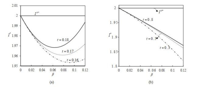
Proposition 5 In the competitive equilibrium of co-existence of green and ordinary production: $(i)$ When $t > \frac{1}{9 k}$ holds, the environmental deterioration decreases with $β$ ; $(i i)$ When $\frac{1}{18 k} < t < \frac{1}{9 k}$ holds, there exists a some $\overset{⌢}{β} \in (0, 1)$ such that the environmental deterioration increases with $β$ if $β ⩾ \overset{⌢}{β}$ , and vice versa; $(i i i)$ the environmental deterioration with co-existence of green and ordinary production is always less than that with no green production, i.e., $I^{*} < I^{N *}$ .

Proposition 5 suggests that although GTA strategy is beneficial to the environment, GTA investment is not the more the better. To demonstrate the interesting interplay of the GTA intensity (i.e.,

β

) and the degree of horizontal differentiation between firms (i.e.,

t

) on environmental damage reduction, we employ a numerical example in Figure 3. Note that when

t

is low (i.e.,

\frac{1}{18 k} < t < \frac{1}{9 k}

), increasing GTA intensity will mitigate the environmental damage only when

β

is lower than a certain threshold. Otherwise, a larger GTA investment will aggravate the environmental damage (see Figure 3(a)). On the other hand, when

t

is high (i.e.,

t > \frac{1}{9 k}

) a stronger GTA intensity always reduces the environmental damage (as shown in Figure 3(b)). Moreover, for a given

β

, a lower degree of horizontal differentiation between firms is always beneficial to mitigate the environmental deterioration (smaller

t

) regardless of the substitutable or complementary effect between GTA strategy and Firm

G

's quality strategy. Thus, from environmental friendly perspective, a social planner should make policies to encourage firms to optimize GTA strategies as well as reduce the degree of horizontal differentiation between firms.

Figure 3 Changes of the environmental impact with $β$ under different $t$ ( $v = 1, k = 0.5, c = 0.8, e = 2$ ). (a) case of $\frac{1}{18 k} < t < \frac{1}{9 k}$ , (b) case of $t > \frac{1}{9 k}$

Full size|PPT slide

Now let us consider effects of GTA strategy on social welfare. Substituting equilibrium consumer surplus, profits and environmental impacts of two types of production, we derive the optimal social welfare as follows.

\begin{array}{rcl} S W^{*} & = & \frac{9 (45 k t - 2) {(k β v)}^{2} + 18 {(9 k t - 1)}^{2} k β v + 36 k {(9 k t - 1)}^{2} (v - c) - {(9 k t - 1)}^{2} (9 k t - 4)}{36 k {(9 k t - 1)}^{2}} \\ - η β^{2} - \frac{e [- 3 k v β^{2} + (2 - β) (9 k t - 1)]}{2 (9 k t - 1)} . \end{array}

(15)

Proposition 6 In equilibrium of the co-existence of green and ordinary production, there exists some $\hat{η}$ such that GTA strategy enhances social welfare, i.e., $S W^{*} ⩾ S W^{N *}$ , if and only if $η < \hat{η}$ , where $\hat{η} = \frac{[(45 k t - 2) v + 6 e (9 k t - 1)] k v}{4 {(9 k t - 1)}^{2}}$ . Moreover, a larger $β$ will increase the social welfare if $η < \hat{η}$ , and vice versa.

Proposition 6 shows that the GTA strategy does not necessarily improve the social welfare. We find that compared with the case of no green production, the GTA strategy implemented by one firm would lead to a higher social welfare only when the GTA efficiency is high enough (i.e.,

η < \hat{η}

). In such a situation, the more the firm invests on GTA strategy, the higher the social welfare is. By contrast, the GTA strategy will lower social welfare when the GTA efficiency is low because the social benefit of GTA strategy cannot cover its social cost. Moreover, note that the cutoff

\hat{η}

\frac{[(45 k t - 2) v + 6 e (9 k t - 1)] k v}{4 {(9 k t - 1)}^{2}}

) depends on the other parameters

k

and

t

. It is straightforward that a decrease in either

k

and

t

would increase this threshold implying that either increasing quality-improving efficiency (i.e., lower

k

) or decreasing the horizontal differentiation between firms (i.e., lower

t

) will support an increase in social welfare in the wake of GTA strategy.

A managerial implication resulted from Proposition 6 is that from the perspective of social optimum, a social planner, on the one hand, need to give incentives to the firm with GTA capability to enhance GTA efficiency and encourage the firm with high GTA efficiency to increase GTA investment; on the other hand, he should also encourage firms to conduct quality-improving innovation as well as try to decrease the horizontal differentiation between firms.

6 Conclusions

Although the environmental damage reduction benefit of the GTA strategy is intuitive, strategic implications of GTA strategy on firms' quality and pricing decisions as well as firms' competitive advantages in terms of gaining profit are not well understood. In this paper, we develop an analytical model to examine both economic and environmental impacts of GTA strategy in duopoly competition. Our analysis indicates that the degree of horizontal differentiation between two firms is a main driver affecting the subtle relationship between the GTA strategy and the green firm's quality strategy. Specifically, a high degree of horizontal differentiation leads to a complementary effect between those two strategies whereas a low degree of horizontal differentiation results in a substitution effect. We find that in the situation of a substitutable (complementary) effect, the quality and price levels as well as the resulted sales of the green firm are always lower (higher) than does its ordinary rival's in equilibrium. Moreover, an increase in GTA intensity would decrease (increase) the green firm's equilibrium outcome but increase (decrease) the ordinary firm's equilibrium outcome.

Furthermore, we highlight that the strategic effect of GTA strategy on firms' profits, consumer surplus and environmental impacts depends on the nuance relationship between GTA strategy and the quality provision of the green firm. The main findings are as follows. First, the firm with GTA strategy never achieve competitive advantages in terms of gaining profit if its quality strategy and GTA strategy are substitutes. Note that the green firm would gain profit advantages only when the GTA efficiency is rather high but the impact of GTA intensity on its profit are not monotonous if its quality strategy and GTA strategy are complementarity. In particular, excessive GTA investment would lead to a decrease in the profit of the green firm. Second, although green consumers would be worse off but ordinary consumers would be better off in the wake of GTA strategy when the GTA strategy exerts a substitutable effect on the quality strategy of the green firm, whereas both of green and ordinary consumers might be better off in the wake of GTA strategy when two strategies are complements. Third, the GTA strategy helps mitigate the environmental damage, but there exists an optimal GTA intensity in the case of substitution effect between the above two strategies. Meanwhile, a lower degree of horizontal differentiation between firms would strengthen the positive impact of GTA strategy on reducing environmental damage. Finally, from the perspective of social optimum, GTA strategy is not always optimal, only when the GTA efficiency is high enough (i.e.,

η < \hat{η}

), GTA strategy would enhance social welfare.

This research also provides several practical implications. First, our findings offer guidelines for the firm with GTA strategy on how to balance its investment on green technology and its quality provision to gain competitive advantage. For example, when the GTA strategy exerts substitutable (complementary) effect on the green firm's quality strategy, the green firm should decrease (increase) its own optimal quality and price levels after joining GTA strategy. Second, our results provide insights to the firm without GTA strategy on how to adjust its quality and price decisions to compete with the firm with GTA strategy. The firm without GTA strategy responds to its competitor's GTA strategy by increasing (decreasing) its own optimal quality and price levels when GTA strategy and the green firm's quality strategy are substitutes (complements). Finally, our results provide managerial insights for social planners on potential policy intervention to promote better quality products and mitigate the environmental deterioration. On the one hand, what the social planner can do is to utilize the policy to enhance a firm's GTA efficiency, i.e., tax incentives, subsidies for green technology innovation, etc. On the other hand, the social planner should also encourage firms to increase quality-improvement efficiency as well as try to decrease the horizontal differentiation between firms.

Although this paper contributes to related literature and practices, there are a number of questions remaining unaddressed, which may be worth future investigation. First, we assume that only one firm implements GTA strategy. In reality, competitive firms usually face the issue of choices of GTA strategy. Thus, we will explore firms' choices of GTA strategy in the context of quality-price competition in the subsequent stage. Second, this paper focuses on fully-covered market, assuming away partial-covered market. In reality, firms encounter either fully-covered or partial-covered market configure. Modeling and examining firms' GTA strategy choices in different market structures and revealing the interaction of market structures, the GTA strategy and firms' actions can be another interesting extension in future research. Finally, we only consider the situation where firms simultaneously enter into the market. However, firms are more likely to conduct the GTA strategy sequentially. As a result, we are going to extend our model to a sequential entry game to analyze firms' strategic behavior in the following research. Further theoretical or empirical research allowing for the above aspects may shed light on their relative influences on green technology adoption strategy.

Acknowledgements

The authors gratefully acknowledge the Editor and anonymous referee for their insightful comments and helpful suggestions that led to a marked improvement of the article.

Appendix

Appendix A

This is the proof for Proposition 1.

Proof From the firms' profit functions shown in (7) and (8), the first-order conditions can be derived as

\begin{array}{l} \frac{\partial Π_{g}^{*} (s_{g}, s_{o})}{\partial s_{g}} = \frac{β v + s_{g} - s_{o} + 3 t}{9 t} - 2 k s_{g}, \end{array}

(A1)

\begin{array}{l} \frac{\partial Π_{o}^{*} (s_{g}, s_{o})}{\partial s_{o}} = \frac{- β v - s_{g} + s_{o} + 3 t}{9 t} - 2 k s_{o}^{} . \end{array}

(A2)

Accordingly, we have the second-order derivatives as follows:

\begin{array}{l} \frac{\partial^{2} Π_{g}^{*} (s_{g}, s_{o})}{\partial {s_{g}}^{2}} = \frac{\partial^{2} Π_{o}^{*} (s_{g}, s_{o})}{\partial {s_{o}}^{2}} = \frac{1}{9 t} - 2 k . \end{array}

(A3)

From (A3), we can derive

\frac{\partial^{2} Π_{g}^{*} (s_{g}, s_{o})}{\partial {s_{g}}^{2}} < 0

and

\frac{\partial^{2} Π_{o}^{*} (s_{g}, s_{o})}{\partial {s_{o}}^{2}} < 0

, if

t > \frac{1}{18 k}

. Thus the solution to the first-order conditions gives the unique maximizer. By solving

\frac{\partial Π_{g}^{*} (s_{g}, s_{o})}{\partial s_{g}} = 0

and

\frac{\partial Π_{o}^{*} (s_{g}, s_{o})}{\partial s_{o}} = 0

, we can derive the optimal quality level of two firms as follows:

\begin{array}{l} \begin{array}{c} s_{g}^{*} = \frac{1}{6 k} + \frac{β v}{2 (9 k t - 1)}, s_{o}^{*} = \frac{1}{6 k} - \frac{β v}{2 (9 k t - 1)} . \end{array} \end{array}

(A4)

Substituting (A4) into (5) and (6), we simplify the optimal prices charged by two firms to

\begin{array}{l} \begin{array}{c} {p_{g}}^{*} = t + c + \frac{3 k t β v}{9 k t - 1}, {p_{o}}^{*} = t + c - \frac{3 k t β v}{9 k t - 1} . \end{array} \end{array}

(A5)

Substituting (A4) and (A5) into (1) and (2), we derive the optimal sales of two firms by some algebra as follows:

\begin{array}{l} \begin{array}{c} {q_{g}}^{*} = \frac{1}{2} + \frac{3 k β v}{2 (9 k t - 1)}, {q_{o}}^{*} = \frac{1}{2} - \frac{3 k β v}{2 (9 k t - 1)} . \end{array} \end{array}

(A6)

Substituting (A4) into (7) and (8), we simplify the firms' profits to

\begin{array}{l} \begin{array}{c} Π_{g}^{*} = \frac{(18 k t - 1) {(3 k β v + 9 k t - 1)}^{2}}{36 k {(9 k t - 1)}^{2}} - η β^{2}, Π_{o}^{*} = \frac{(18 k t - 1) {(- 3 k β v + 9 k t - 1)}^{2}}{36 k {(9 k t - 1)}^{2}} . \end{array} \end{array}

(A7)

Note that the necessary condition for a competitive equilibrium must satisfy

0 < {q_{g}}^{*} < 1, 0 < {q_{o}}^{*} < 1

, which leads to

β < \frac{| 9 k t - 1 |}{3 k v}

implying that the GTA intensity should not be too high. Otherwise, the firm without GTA will be squeezed out of the market.

Appendix B

This is the proof for Corollary 2.

Proof From the results in Proposition 1, taking the first-order derivative with respect to

β

gives that

\frac{\partial s_{g}^{*}}{\partial β} = \frac{v}{2 (9 k t - 1)}, \frac{\partial s_{o}^{*}}{\partial β} = - \frac{v}{2 (9 k t - 1)}, \frac{\partial {p_{g}}^{*}}{\partial β} = \frac{3 k t v}{9 k t - 1}, \frac{\partial {p_{o}}^{*}}{\partial β} = - \frac{3 k t β v}{9 k t - 1}

\frac{\partial {q_{g}}^{*}}{\partial β} = \frac{3 k v}{2 (9 k t - 1)}

, and

\frac{\partial {q_{o}}^{*}}{\partial β} = - \frac{3 k v}{2 (9 k t - 1)}

. It is straightforward that

\frac{\partial {s_{g}}^{*}}{\partial β} > 0, \frac{\partial {s_{o}}^{*}}{\partial β} < 0, \frac{\partial {p_{g}}^{*}}{\partial β} > 0, \frac{\partial {p_{o}}^{*}}{\partial β} < 0, \frac{\partial q_{g}^{*}}{\partial β} > 0, \frac{\partial q_{o}^{*}}{\partial β} < 0

9 k t - 1 > 0

, i.e.,

t > \frac{1}{9 k}

, whereas

\frac{\partial {s_{g}}^{*}}{\partial β} < 0, \frac{\partial {s_{o}}^{*}}{\partial β} > 0, \frac{\partial {p_{g}}^{*}}{\partial β} < 0, \frac{\partial {p_{o}}^{*}}{\partial β} > 0, \frac{\partial q_{g}^{*}}{\partial β} < 0, \frac{\partial q_{o}^{*}}{\partial β} > 0

, if

9 k t - 1 < 0

, i.e.,

t < \frac{1}{9 k}

Appendix C

This is the proof for Proposition 2.

Proof To solve the difference of

Π_{g}^{*}

and

Π_{o}^{*}

, we have

Π_{g}^{*} - Π_{o}^{*} = \frac{β v (18 k t - 1)}{3 (9 k t - 1)} - η β^{2}

. We first consider the case of

\frac{1}{18 k} < t < \frac{1}{9 k}

. When

\frac{1}{18 k} < t < \frac{1}{9 k}

, it is straightforward that

Π_{g}^{*} - Π_{o}^{*} = \frac{β v (18 k t - 1)}{3 (9 k t - 1)} - η β^{2} < 0

since

β > 0

. Accordingly, taking the first-order derivatives with respect to

β

, we have

\frac{\partial Π_{g}^{*}}{\partial β} = \frac{(3 β v + 9 k t - 1) (18 k t - 1) v}{6 {(9 k t - 1)}^{2}} - 2 η β < 0

and

\frac{\partial Π_{o}^{*}}{\partial β} = \frac{(3 β v - 9 k t + 1) (18 k t - 1) v}{6 {(9 k t - 1)}^{2}} > 0

, since

β < \frac{| 9 k t - 1 |}{3 k v}

Now we consider the case of

t > \frac{1}{9 k}

. For ease of exposition, we define

Δ Π = Π_{g}^{*} - Π_{o}^{*}

, and then derive

Δ Π = \frac{β v (18 k t - 1)}{3 (9 k t - 1)} - η β^{2}

. It is not hard to derive that

Δ Π = 0

when

β = 0

and

β = \frac{(18 k t - 1) v}{3 η (9 k t - 1)}

. Since

\frac{\partial^{2} Δ Π}{\partial β^{2}} = - 2 η < 0

, we obtain that

Δ Π

is concave in

β

. In addition, we obtain

β^{*} = \frac{(18 k t - 1) v}{6 η (9 k t - 1)}

from the first-order condition

\frac{\partial Δ Π}{\partial β} = \frac{v (18 k t - 1)}{3 (9 k t - 1)} - 2 η β = 0

. On basis of the above analysis, we can derive that

Δ Π ⩾ 0

when

β \in (0, \frac{(18 k t - 1) v}{3 η (9 k t - 1)}]

holds, and

Δ Π < 0

when

β > \frac{(18 k t - 1) v}{3 η (9 k t - 1)}

holds.

In what follows, we prove the effect of on both firms' optimal profits. We have the first-order derivatives as follows:

\begin{array}{rcl} \begin{matrix} \frac{\partial Π_{o}^{*}}{\partial β} = \frac{(3 β v - 9 k t + 1) (18 k t - 1) v}{6 {(9 k t - 1)}^{2}} < 0, \end{matrix} \end{array}

\begin{array}{rcl} \begin{matrix} \frac{\partial Π_{g}^{*}}{\partial β} = \frac{(3 β v + 9 k t - 1) (18 k t - 1) v}{6 {(9 k t - 1)}^{2}} - 2 η β . \end{matrix} \end{array}

Differentiating

Π_{g}^{*}

with respect to

β

twice gives to

\frac{\partial^{2} Π_{g}^{*}}{\partial β^{2}} = \frac{(18 k t - 1) v^{2}}{2 {(9 k t - 1)}^{2}} - 2 η

. According to the assumption of

η > \frac{(18 k t - 1) v^{2}}{4 {(9 k t - 1)}^{2}}

, it is straightforward that

Π_{g}^{*}

is concave in

β

. Solving

\frac{\partial Π_{g}^{*}}{\partial β} = 0

gives to

β^{*} = \frac{(9 k t - 1) (18 k t - 1) v}{3 [4 η {(9 k t - 1)}^{2} - (18 k t - 1) v^{2}]}

. Since

t > \frac{1}{9 k}

, we have

β^{*} > 0

for

η > \frac{(18 k t - 1) v^{2}}{4 {(9 k t - 1)}^{2}}

and

β^{*} < 0

for

η < \frac{(18 k t - 1) v^{2}}{4 {(9 k t - 1)}^{2}}

. Therefore, we have

\frac{\partial Π_{g}^{*}}{\partial β} > 0

for

β < β^{*}

and

\frac{\partial Π_{g}^{*}}{\partial β} < 0

for

β > β^{*} > 0

Appendix D

This is the proof for Proposition 3.

Proof From (11), the first-order conditions can be derived as

\begin{array}{l} \frac{\partial {C S}_{g}^{*}}{\partial β} = \frac{3 k v [(21 k t - 2) β v + (9 k t - 1) (2 (v - c) + t)]}{4 {(9 k t - 1)}^{2}} . \end{array}

(A8)

Accordingly, we have the second-order derivatives as follows:

\begin{array}{l} \frac{\partial^{2} {C S}_{g}^{*}}{\partial β^{2}} = \frac{3 k v^{2} (21 k t - 2)}{4 {(9 k t - 1)}^{2}} . \end{array}

(A9)

From (9), we obtain

\frac{\partial^{2} {C S}_{g}^{*}}{\partial β^{2}} > 0

(i.e.,

{C S}_{g}^{*}

is convex with respect to

β

) for

21 k t - 2 > 0

and

\frac{\partial^{2} {C S}_{g}^{*}}{\partial β^{2}} < 0

(i.e.,

{C S}_{g}^{*}

is concave with respect to

β

) for

21 k t - 2 < 0

. Solving

\frac{\partial {C S}_{g}^{*}}{\partial β} = 0

, we get

\hat{β} = - \frac{(9 k t - 1) (2 (v - c) + t)}{(21 k t - 2) v}

. Therefore, we can discuss the following three cases:

(ⅰ) When

t > \frac{1}{9 k}

, it always leads to

t > \frac{2}{21 k}

. Thus, we have

\hat{β} < 0

. Since

{C S}_{g}^{*}

is convex with respect to

β

, it is straightforward that

\frac{\partial {C S}_{g}^{*}}{\partial β} > 0

for

β > \hat{β}

and

\frac{\partial {C S}_{g}^{*}}{\partial β} < 0

for

β < \hat{β}

. Given

β > 0

β

always satisfies

β > \hat{β}

, therefore, we always have

\frac{\partial {C S}_{g}^{*}}{\partial β} > 0

in the case of

t > \frac{1}{9 k}

;

(ⅱ) When

\frac{2}{21 k} > t > \frac{1}{18 k}

, it leads to

\hat{β} < 0

. Since

{C S}_{g}^{*}

is convex with respect to

β

, it is straightforward that

\frac{\partial {C S}_{g}^{*}}{\partial β} < 0

for

β < \hat{β}

and

\frac{\partial {C S}_{g}^{*}}{\partial β} > 0

for

β > \hat{β}

. Comparing

\hat{β}

and

\bar{β} = \frac{| 9 k t - 1 |}{3 k v}

, we obtain

\bar{β} - \hat{β} = \frac{(9 k t - 1) [- 2 (9 k t - 1) + 6 k (v - c)]}{3 k v (21 k t - 2)} < 0

, namely,

\bar{β} < \hat{β}

, implying that all

β \in (0, \bar{β})

is lower than

\hat{β}

. Therefore, we always have

\frac{\partial {C S}_{g}^{*}}{\partial β} < 0

in this case;

(ⅲ) When

\frac{2}{21 k} > t > \frac{1}{18 k}

, it leads to

\hat{β} < 0

. Since

{C S}_{g}^{*}

is concave with respect to

β

, we have

\frac{\partial {C S}_{g}^{*}}{\partial β} < 0

for

β > \hat{β}

and

\frac{\partial {C S}_{g}^{*}}{\partial β} > 0

for

β < \hat{β}

. Given

β > 0

, it is unreasonable for

β < \hat{β} < 0

, therefore, we have

\frac{\partial {C S}_{g}^{*}}{\partial β} < 0

because

β

always satisfies

β > 0 > \hat{β}

In summary, we can derive that

\frac{\partial {C S}_{g}^{*}}{\partial β} > 0

for

t > \frac{1}{9 k}

and

\frac{\partial {C S}_{g}^{*}}{\partial β} < 0

for

\frac{1}{9 k} > t > \frac{1}{18 k}

Appendix E

This is the proof for Proposition 4.

Proof From (12), the first-order conditions can be derived as

\begin{array}{l} \frac{\partial {C S}_{o}^{*}}{\partial β} = \frac{- v [3 k (15 k t - 2) β v - (9 k t - 1) (15 k t - 2 - 6 k (v - c))]}{4 {(9 k t - 1)}^{2}} . \end{array}

(A10)

Accordingly, we have the second-order derivatives as follows:

\begin{array}{l} \frac{\partial^{2} {C S}_{o}^{*}}{\partial β^{2}} = - \frac{3 k v^{2} (15 k t - 2)}{4 {(9 k t - 1)}^{2}} . \end{array}

(A11)

From (A11), we obtain

\frac{\partial^{2} {C S}_{o}^{*}}{\partial β^{2}} \leq 0

for

15 k t - 2 > 0

and

\frac{\partial^{2} {C S}_{o}^{*}}{\partial β^{2}} > 0

for

15 k t - 2 < 0

. Solving

\frac{\partial {C S}_{o}^{*}}{\partial β} = 0

, it leads to

\hat{β} = \frac{(9 k t - 1) [15 k t - 2 - 6 k (v - c)]}{3 k v (15 k t - 2)}

. Then four possible conditions left in accordance with the range of

t

(ⅰ) When

t \geq \frac{2 + 6 k (v - c)}{15 k}

, it leads to

\frac{\partial^{2} {C S}_{o}^{*}}{\partial β^{2}} \leq 0

, which implies that

{C S}_{o}^{*}

is concave in

β

. Since

t \geq \frac{2 + 6 k (v - c)}{15 k}

, it is straightforward that

\hat{β} \geq 0

. Moreover, we have

\frac{\partial {C S}_{o}^{*}}{\partial β} \geq 0

for

β \leq \hat{β}

and

\frac{\partial {C S}_{o}^{*}}{\partial β} < 0

for

β > \hat{β}

. Additionally, comparing

\hat{β}

with

\bar{β} = \frac{| 9 k t - 1 |}{3 k v}

, we obtain

\bar{β} - \hat{β} = \frac{6 k (9 k t - 1) (v - c)}{3 k v (15 k t - 2)} > 0

;

(ⅱ) When

\frac{2 + 6 k (v - c)}{15 k} > t \geq \frac{2}{15 k}

{C S}_{o}^{*}

is also concave in

β

and

\hat{β} < 0

. It is straightforward that

\frac{\partial {C S}_{o}^{*}}{\partial β} \geq 0

for

β \leq \hat{β}

and

\frac{\partial {C S}_{o}^{*}}{\partial β} < 0

for

β > \hat{β}

. Since

β > 0

, we always have

\frac{\partial {C S}_{o}^{*}}{\partial β} < 0

;

(ⅲ) When

\frac{2}{15 k} > t \geq \frac{1}{9 k}

, it leads to the case that

{C S}_{o}^{*}

is convex in

β

due to

\frac{\partial^{2} {C S}_{o}^{*}}{\partial β^{2}} > 0

, and

\hat{β} > 0

. It is straightforward that

\frac{\partial {C S}_{o}^{*}}{\partial β} \leq 0

for

β \leq \hat{β}

and

\frac{\partial {C S}_{o}^{*}}{\partial β} > 0

for

β > \hat{β}

. Comparing

\hat{β}

with

\bar{β} = \frac{| 9 k t - 1 |}{3 k v}

, we obtain

\bar{β} - \hat{β} = \frac{6 k (9 k t - 1) (v - c)}{3 k v (15 k t - 2)} < 0

, i.e.,

\bar{β} < \hat{β}

, which means that

β

is always lower than

\hat{β}

in equilibrium. Therefore, we have

\frac{\partial {C S}_{o}^{*}}{\partial β} < 0

;

(ⅳ) When

\frac{1}{9 k} > t > \frac{1}{18 k}

, it leads to the case that

{C S}_{o}^{*}

is convex in

β

due to

\frac{\partial^{2} {C S}_{o}^{*}}{\partial β^{2}} > 0

, and

\hat{β} < 0

. It is straightforward that

\frac{\partial {C S}_{o}^{*}}{\partial β} \leq 0

for

β \leq \hat{β}

and

\frac{\partial {C S}_{o}^{*}}{\partial β} > 0

for

β > \hat{β}

. Given

β > 0

, we always have

\frac{\partial {C S}_{o}^{*}}{\partial β} > 0

Appendix F

This is the proof for Proposition 5.

Proof Substituting optimal quantities shown in Proposition 1 into (14), we obtain

\begin{array}{l} I^{*} = \frac{e [- 3 k v β^{2} + (2 - β) (9 k t - 1)]}{2 (9 k t - 1)} . \end{array}

(A12)

Substituting

β = 0

into (A12), we derive the optimal environment impact in the case of non-GTA strategy, that is,

I^{N *} = e

Define

Δ I = I^{*} - I^{N *}

. Substituting (A11) and (A12) into the expression of

Δ I

, we derive

\begin{array}{l} Δ I = - \frac{(3 k β v + 9 k t - 1) β e}{2 (9 k t - 1)} . \end{array}

(A13)

It is straightforward that

Δ I < 0

whenever

9 k t - 1 > 0

and

9 k t - 1 < 0

In what follows, we prove the effect of the GTA intensity (

β

) on the optimal environmental impact (

I^{*}

). Differentiating

I^{*}

with respect to

β

gives

\begin{array}{l} \frac{\partial I^{*}}{\partial β} = - \frac{e [6 k β v + (9 k t - 1)]}{2 (9 k t - 1)} . \end{array}

(A14)

Next, we differentiate

I^{*}

with respect to

β

twice to get

\begin{array}{l} \frac{\partial^{2} I^{*}}{\partial β^{2}} = - \frac{3 k v e}{(9 k t - 1)} . \end{array}

(A15)

It is straightforward that

\frac{\partial^{2} I^{*}}{\partial β^{2}} < 0

for

9 k t - 1 > 0

and

\frac{\partial^{2} I^{*}}{\partial β^{2}} > 0

for

9 k t - 1 < 0

. When

9 k t - 1 > 0

, we derive that

I^{*}

is concave in

β

due to

\frac{\partial^{2} I^{*}}{\partial β^{2}} < 0

. From (A14), it is straightforward that

\frac{\partial I^{*}}{\partial β} < 0

for

9 k t - 1 > 0

, i.e.,

t > \frac{1}{9 k}

. On the other hand, when

9 k t - 1 < 0

, we derive that

I^{*}

is convex in

β

due to

\frac{\partial^{2} I^{*}}{\partial β^{2}} > 0

. By solving

\frac{\partial I^{*}}{\partial β} = 0

, we obtain the optimal

\overset{⌢}{β} = - \frac{(9 k t - 1)}{6 k v} > 0

. Therefore, we obtain that

\frac{\partial I^{*}}{\partial β} \geq 0

for

β \geq \overset{⌢}{β}

and

\frac{\partial I^{*}}{\partial β} < 0

for

β < \overset{⌢}{β}

. In addition, by comparing

\overset{⌢}{β}

with

\bar{β} = \frac{| 9 k t - 1 |}{3 k v}

, we have

\overset{⌢}{β} < \bar{β}

Appendix G

This is the proof for Proposition 6.

Proof We first compare the social welfare with no green production and that with the co-existence of green and ordinary production. For ease of exposition, we define

Δ S W = S W^{*} - S W^{^{N *}}

, where

S W^{N *}

is social welfare with no green production, i.e.,

β = 0

. After some simple algebra, we obtain

\begin{array}{l} Δ S W = \frac{(45 k t - 2) k β^{2} v^{2} + 2 {(9 k t - 1)}^{2} β v}{4 {(9 k t - 1)}^{2}} + \frac{e β (3 k β v + 9 k t - 1)}{2 (9 k t - 1)} - η β^{2} . \end{array}

(A16)

From (A16), it is straightforward that

Δ S W = 0

when

β^{o} = \frac{{(9 k t - 1)}^{2} (v + e)}{4 η {(9 k t - 1)}^{2} - [(45 k t - 2) v + 6 e (9 k t - 1)] k v}

Differentiating

Δ S W

with respect to

β

gives

\begin{array}{l} \frac{\partial Δ S W}{\partial β} = \frac{v [(45 k t - 2) k β v + {(9 k t - 1)}^{2}]}{2 {(9 k t - 1)}^{2}} + \frac{e (6 k β v + 9 k t - 1)}{2 (9 k t - 1)} - 2 η β . \end{array}

(A17)

Differentiating

Δ S W

with respect to

β

twice gives

\begin{array}{l} \frac{\partial^{2} Δ S W}{\partial β^{2}} = \frac{(45 k t - 2) k v^{2}}{2 {(9 k t - 1)}^{2}} + \frac{3 k v e}{(9 k t - 1)} - 2 η . \end{array}

(A18)

It is straightforward that

\frac{\partial^{2} Δ S W}{\partial β^{2}} < 0

η > \hat{η} = \frac{[(45 k t - 2) v + 6 e (9 k t - 1)] k v}{4 {(9 k t - 1)}^{2}}

, which implies that

Δ S W

is concave in

β

. Otherwise,

\frac{\partial^{2} Δ S W}{\partial β^{2}} > 0

, if

η < \hat{η}

, which implies that

Δ S W

is convex in

β

. To avoid triviality, we neglect the condition of

η = \hat{η}

. By solving

\frac{\partial Δ S W}{\partial β} = 0

, we get

β^{*} = \frac{(v + e) {(9 k t - 1)}^{2}}{4 η {(9 k t - 1)}^{2} - [(45 k t - 2) v + 6 e (9 k t - 1)] k v}

. Thus, we have

β^{*} < 0

for

η < \hat{η}

and

β^{*} > 0

for

η > \hat{η}

Since

Δ S W

is concave in

β

in the case of

η > \hat{η}

, it is straightforward that

Δ S W

is maximal at the point

β^{*}

. Meanwhile

Δ S W |_{β = β *} = 0

, since

β^{*} = β^{o}

, which implies that

Δ S W \leq 0

. In other words,

S W^{*} \leq S W^{^{N *}}

η > \hat{η}

holds. On the other hand, since

Δ S W

is convex in

β

in the case of

η < \hat{η}

, it is straightforward that

Δ S W

is minimal at the point

β^{*}

, here

Δ S W |_{β = β *} = 0

due to

β^{*} = β^{o}

, which implies that

Δ S W \geq 0

Next we prove the effects of

β

on the social welfare

S W^{*}

in equilibrium.

Differentiating

S W^{*}

with respect to

β

gives

\begin{array}{l} \frac{\partial S W^{*}}{\partial β} = \frac{v [(45 k t - 2) k β v + {(9 k t - 1)}^{2}]}{2 {(9 k t - 1)}^{2}} + \frac{e (6 k β v + 9 k t - 1)}{2 (9 k t - 1)} - 2 η β . \end{array}

(A19)

Differentiating

S W^{*}

with respect to

β

twice gives

\begin{array}{l} \frac{\partial^{2} S W^{*}}{\partial β^{2}} = \frac{(45 k t - 2) k v^{2}}{2 {(9 k t - 1)}^{2}} + \frac{3 k v e}{(9 k t - 1)} - 2 η . \end{array}

(A20)

Therefore, we can derive

\frac{\partial^{2} S W^{*}}{\partial β^{2}} < 0

for

η > \hat{η}

and

\frac{\partial^{2} S W^{*}}{\partial β^{2}} > 0

for

η < \hat{η}

. Solving

\frac{\partial S W^{*}}{\partial β} = 0

, we have

\begin{array}{l} β^{*} = \frac{(v + e) {(9 k t - 1)}^{2}}{4 η {(9 k t - 1)}^{2} - [(45 k t - 2) v + 6 e (9 k t - 1)] k v} . \end{array}

(A21)

It is straightforward that

β^{*} < 0

for

η < \hat{η}

and

β^{*} > 0

for

η > \hat{η}

. In addition, if

η > \hat{η}

S W^{*}

is concave in

β

. Therefore, we can derive that

S W^{*}

is increasing in

β

for

β < β^{*}

and decreasing in

β

for

β \geq β^{*}

. Since

β

is always larger than zero,

S W^{*}

is always decreasing in

β

η > \hat{η}

holds. On the other hand, if

η < \hat{η}

, then we have

\frac{\partial^{2} S W^{*}}{\partial β^{2}} > 0

, implying that

S W^{*}

is convex in

β

. Therefore, we can derive that

S W^{*}

is decreasing in

β

for

β < β^{*}

and increasing in

β

for

β \geq β^{*}

. Since

β

is always larger than zero,

S W^{*}

is always increasing in

β

η < \hat{η}

holds.

References

Publishing order | Descend order by publishing year | Descend order by cited within

1	Cohen M C, Lobel R, Perakis G. The impact of demand uncertainty on consumer subsidies for green technology adoption. Management Science, 2016, 63(5): 1235- 1258. Cited in this article [1]

2	Lin R J, Tan K H, Geng Y. Market demand green product innovation and firm performance: Evidence from Vietnam motorcycle industry. Journal of Cleaner Production, 2013, 40, 101- 107. https://doi.org/10.1016/j.jclepro.2012.01.001 Cited in this article [1]

3	Du S F, Tang W Z, Song M L. Low-carbon production with low-carbon premium in cap-and-trade regulation. Journal of Cleaner Production, 2016, 134, 652- 662. https://doi.org/10.1016/j.jclepro.2016.01.012 Cited in this article [3]

4	Tully S M, Winer R S. The role of the beneficiary in willing to pay for socially responsible products: A meta-analysis. Journal of Retailing, 2014, 90(2): 255- 274. https://doi.org/10.1016/j.jretai.2014.03.004 Cited in this article [1]

5	Bhattacharya G C, Sen S. Doing better at doing good: When, why and how consumers respond to corporate social initiatives. California Management Review, 2004, 47(1): 9- 24. https://doi.org/10.2307/41166284 Cited in this article [1]

6	Servaes H, Tamayo A. The impact of corporate social responsibility on firm value: The role of customer awareness. Management Science, 2013, 59(5): 1045- 1061.

7	Haw K L, Winterich K P, Naylor R W. Seeing the world through GREEN-tinted glasses: Green consumption values and responses to environmentally friendly products. Journal of Consumer Psychology, 2014, 24(3): 336- 354. https://doi.org/10.1016/j.jcps.2013.11.002 Cited in this article [1]

8	Krass D, Nedorezov T, Ovchinnikov A. Environmental taxes and the choice of green technology. Production and Operations Management, 2013, 22(5): 1035- 1055. Cited in this article [1]

9	Ginsberg J M, Bloom P N. Choosing the right green marketing strategy. Sloan Management Review, 2004, 46(1): 79- 84. Cited in this article [1]

10	Gu W J, Chhajed D, Petruzzi N C, et al. Quality design and environmental implications of green consumerism in remanufacturing. International Journal of Production Economics, 2015, 162, 55- 69. https://doi.org/10.1016/j.ijpe.2014.12.040 Cited in this article [4]

11	Andre F J, Gonzalez P, Porteiro N. Strategic quality competition and the porter hypothesis. Journal of Environmental Economics and Management, 2009, 57(2): 182- 194. https://doi.org/10.1016/j.jeem.2008.07.002 Cited in this article [1]

12	Yalabik B, Fairchild R J. Customer regulatory and competitive pressure as drivers of environmental innovation. International Journal of Production Economics, 2011, 131, 519- 527. https://doi.org/10.1016/j.ijpe.2011.01.020

13	Liu Z, Anderson T D, Cruz J M. Consumer environmental awareness and competition in two-stage supply chains. European Journal of Operational Research, 2012, 218, 602- 613. https://doi.org/10.1016/j.ejor.2011.11.027

14	Bi G, Jin M, Liang L, et al. Environmental subsidy and the choice of green technology in the presence of green consumers. Annals of Operations Research, 2017, 255(1-2): 547- 568.

15	Yu Y, Han X, Hu G. Optimal production for manufacturers considering consumer environmental awareness and green subsidies. International Journal of Production Economics, 2016, 182, 397- 408. https://doi.org/10.1016/j.ijpe.2016.09.014 Cited in this article [1]

16	Galbreth M R, Ghosh B. Competition and sustainability: The impact of consumer awareness. Decision Science, 2013, 44(1): 127- 159. https://doi.org/10.1111/j.1540-5915.2012.00395.x Cited in this article [1]

17	Zhou Y. The role of green customers under competition: A mixed blessing?, , 170:857-866. Journal of Cleaner Production, 2018, 170, 857- 866. https://doi.org/10.1016/j.jclepro.2017.09.155 Cited in this article [3]

18	Mussa M, Rosen S. Monopoly and product quality. Journal of Economic Theory, 1978, 18(2): 301- 317. https://doi.org/10.1016/0022-0531(78)90085-6 Cited in this article [1]

19	Moorthy K S, Png I P L. Market segmentation cannibalization and the timing of product introductions. Marketing Science, 1992, 38(2): 345- 359.

20	Desai P. Quality segmentation in spatial markets: When does cannibalization affect product line design?. Marketing Science, 2001, 20(3): 265- 283. https://doi.org/10.1287/mksc.20.3.265.9767 Cited in this article [1]

21	Wattal S, Telang R, Mukhopadhyay T. Information personalization in a two-dimensional product differentiation model. Journal of Management Information Systems, 2009, 26(2): 69- 95. Cited in this article [1]

22	Ma P, Zhang C, Hong X P, et al. Pricing decisions for substitutable products with green manufacturing in a competitive supply chain. Journal of Cleaner Production, 2018, 183, 618- 640. Cited in this article [1]

23	Hotelling H. Stability in competion. The Economic Journal, 1929, 39(153): 41- 57. Cited in this article [1]

24	Wiengarten F, Pagell M. The importance of quality management for the success of environmental management iniatives. International Journal of Production Economics, 2012, 146, 106- 197. Cited in this article [1]

25	Brekke K R, Siciliani L, Straume O R. Qualitu competition with profit constraints. Journal of Economic Behavior & Organization, 2012, 84(2): 642- 659.

26	Shi H Y, Liu Y C, Petruzzi N. Consumer heterogeneity product quality and distribution channel. Management Science, 2013, 59(5): 1162- 1176. Cited in this article [1]

27	Zhang F Q, Zhang R Y. Trade-in remanufacturing customer purchasing behavior and government policy. Manufacturing & Service Operations Management, 2018, 20(4): 601- 616. Cited in this article [1]

28	Örsdemir A, Kemahlioglu-Ziya E, Parlaktürk A K. Competitive quality choice and remanufacturing. Production and Operations Management, 2013, 23(1): 48- 64. Cited in this article [1]

PDF(310 KB)

374

Accesses

Citation

Detail

Sections

Recommended

Abstract
Key words
Cite this article
1 Introduction
2 Literature Review
3 Model Descriptions and Notations
Table 1 Notations for variables and parameters
4 Equilibrium Analysis
5 Welfare Analysis
Figure 1 Changes of consumer surplus for the firm without GTA strategy with $β$ under different $t$ ( $v = 3$ , $k = 0.5$ ). (a) when GTA strategy and Firm G's quality strategy are substitutes (i.e., $0.11 < t < 0.22$ ), (b) when GTA strategy and the green firm's quality provision are complements (i.e., $t > 0.22$ )
Figure 2 Changes of consumer surplus for the firm without GTA strategy with $β$ under different $t$ ( $v = 3$ , $k = 0.5$ ). (a) Case of $t > \frac{2 + 6 k (v - c)}{15 k}$ , (b) Case of $t \in (\frac{1}{9 k}, \frac{2 + 6 k (v - c)}{15 k})$ , and (c) case of $t \in (\frac{1}{18 k}, \frac{1}{9 k})$
Figure 3 Changes of the environmental impact with $β$ under different $t$ ( $v = 1, k = 0.5, c = 0.8, e = 2$ ). (a) case of $\frac{1}{18 k} < t < \frac{1}{9 k}$ , (b) case of $t > \frac{1}{9 k}$
6 Conclusions
Acknowledgements
Appendix
Appendix A
Appendix B
Appendix C
Appendix D
Appendix E
Appendix F
Appendix G
References

Received	Accepted	Published
2020-10-20	2021-04-01	2021-10-25
Issue Date
2021-10-25

Please choose a citation manager

Content to export

Abstract

Key words

Cite this article

1 Introduction

2 Literature Review

3 Model Descriptions and Notations

Table 1 Notations for variables and parameters

4 Equilibrium Analysis

5 Welfare Analysis

Figure 2 Changes of consumer surplus for the firm without GTA strategy with $β$ under different $t$ ( $v = 3$ , $k = 0.5$ ). (a) Case of $t > \frac{2 + 6 k (v - c)}{15 k}$ , (b) Case of $t \in (\frac{1}{9 k}, \frac{2 + 6 k (v - c)}{15 k})$ , and (c) case of $t \in (\frac{1}{18 k}, \frac{1}{9 k})$

Figure 3 Changes of the environmental impact with $β$ under different $t$ ( $v = 1, k = 0.5, c = 0.8, e = 2$ ). (a) case of $\frac{1}{18 k} < t < \frac{1}{9 k}$ , (b) case of $t > \frac{1}{9 k}$

6 Conclusions

Acknowledgements

Appendix

Appendix A

Appendix B

Appendix C

Appendix D

Appendix E

Appendix F

Appendix G

{{custom_sec.title}}

{{custom_sec.title}}

References

{{custom_fnGroup.title_en}}

Footnotes

Share

模态框（Modal）标题

Please choose a citation manager

Content to export

Abstract

Key words

Cite this article

1 Introduction

2 Literature Review

3 Model Descriptions and Notations

Table 1 Notations for variables and parameters

4 Equilibrium Analysis

5 Welfare Analysis

Figure 1 Changes of consumer surplus for the firm without GTA strategy with β under different t (v=3, k=0.5). (a) when GTA strategy and Firm G's quality strategy are substitutes (i.e., 0.11<t<0.22), (b) when GTA strategy and the green firm's quality provision are complements (i.e., t>0.22)

Figure 2 Changes of consumer surplus for the firm without GTA strategy with β under different t (v=3, k=0.5). (a) Case of t>2+6k(v−c)15k, (b) Case of t∈(19k,2+6k(v−c)15k), and (c) case of t∈(118k,19k)

Figure 3 Changes of the environmental impact with β under different t (v=1, k=0.5, c=0.8, e=2). (a) case of 118k<t<19k, (b) case of t>19k

6 Conclusions

Acknowledgements

Appendix

Appendix A

Appendix B

Appendix C

Appendix D

Appendix E

Appendix F

Appendix G

{{custom_sec.title}}

{{custom_sec.title}}

References

{{custom_fnGroup.title_en}}

Footnotes

Figure 2 Changes of consumer surplus for the firm without GTA strategy with $β$ under different $t$ ( $v = 3$ , $k = 0.5$ ). (a) Case of $t > \frac{2 + 6 k (v - c)}{15 k}$ , (b) Case of $t \in (\frac{1}{9 k}, \frac{2 + 6 k (v - c)}{15 k})$ , and (c) case of $t \in (\frac{1}{18 k}, \frac{1}{9 k})$

Figure 3 Changes of the environmental impact with $β$ under different $t$ ( $v = 1, k = 0.5, c = 0.8, e = 2$ ). (a) case of $\frac{1}{18 k} < t < \frac{1}{9 k}$ , (b) case of $t > \frac{1}{9 k}$