1 Introduction
The existing literature has emphasised that uncertainty can not only directly affect firms' behaviour, with regard to trade, investment and innovation, but also change the sensitivity of firms to credit constraints, trade barriers and other related factors, therefore, have a far-reaching impact on the economy
[1, 2]. Therefore, different from the impact of policy change itself, the impact of policy uncertainty is more likely to interact with other economic variables, resulting in higher-order effects. However, the studies above are mainly focused on the macro-economic level, and most of the existing micro-level trade literature still focuses on the direct economic effects of policy uncertainty, simplifying or ignoring the higher-order effects caused by the interaction of policy uncertainty and other economic variables.
This paper will focus on the higher-order effects of trade policy uncertainty (TPU), specifically the interaction of such uncertainty and credit constraint heterogeneity on firms' export behaviour. There are two reasons why the heterogeneity of credit constraints should be included in the analytical framework. First, credit constraints have always been an important issue in the field of trade studies and, significantly affect firms' export behaviour and trade welfare effects through trade costs
[3]. Second, apart from the credit constraint heterogeneity caused by different asset scales and productivity, differences in firm ownership and managers' experience will also lead to different credit constraints
[4, 5]. Moreover, compared with domestic firms, export-oriented firms have easier access to bank finance
[6]; that is, firms are faced with significant heterogeneity in terms of credit constraints in reality.
This paper develops a simple trade model of heterogeneous firms, which incorporates exogenous industry-level and endogenous firm-level credit constraint heterogeneity and reveals the interaction mechanisms of TPU and credit constraint heterogeneity on exporters' behaviour. On the one hand, the level of credit constraints determined by the exogenous characteristics of industries will affect the fixed costs of exports, magnifying the impact of TPU on firms' exports; that is, in industries with more serious credit constraints, changes in TPU will have a greater impact on exports. On the other hand, in a specific industry, inefficient firms will endogenously choose export patterns with lower levels of credit constraints at the expense of variable profits, so for such firms, the impact of industry-level credit constraints is greater, and they are greatly affected by the interaction of industry-level credit constraints and TPU.
Based on China's micro-level trade data from the years 2000 to 2013, we adopt a difference-in-difference-in-differences (DDD) method to empirically identify the main predictions and mechanisms of the model. First, we use financial vulnerability data for 24 at the International Standard Industrial Classification (ISIC) 3-digit industry level and 9 at the ISIC 4-digit industry level, calculated by Kroszner, et al.
[7] as a proxy for industry-level credit constraints. The index is calculated by using data on American listed companies from the years 1980 to 1999, which is, on the one hand, helpful in terms of avoiding reverse causal relationships between firms' exports and credit constraints in the empirical regressions; on the other hand, it also helps to isolate the impact of TPU changes on China's industry-level credit constraints and, therefore better meets the exogeneity demand for industrial credit constraints in the theoretical model. Second, consistent with Handley and Limão
[8], we use the historical event of "after China's accession to the World Trade Organization (WTO), the United States granted China Permanent Normal Trade Relations (PNTR) status" as a basis for identifying changes in TPU in the theoretical model. As is mentioned in Handley and Limão
[9], the uncertainty based on tariff adjustment will not change as frequently as the uncertainty caused by demand fluctuations, so it is not easy to directly affect firms' pricing behaviour. Moreover, the relationship between the TPU index and the credit constraints that fluctuates more frequently is also weak, thus isolating the endogenous impacts of uncertainty on credit constraints. In sum, the proxy for TPU constructed by this method is consistent with the assumption of TPU in our theoretical model. Finally, due to the fact that the level of the explanatory variables in the regressions is higher than that of the explained variable, according to Angrist and Pischke
[10], we calculate the clustering standard errors at the industry level.
The empirical results show that under the control of some factors, such as tariff reduction, market supply and demand, a TPU decline will significantly promote the export scales and the export extensive margin of industries, and such an effect will be greater in those industries with more serious credit constraints. After adding more control variables and using different TPU indexes, the results remain robust. Finally, for industries with higher fixed costs, the interaction of TPU and industry-level credit constraints is greater. In general, the empirical results support the main predictions of the theoretical model.
There are two main strands of literature closely related to our study. The first strand focuses on the relationship between TPU and exports. With regard to theoretical research, Handley
[11] introduces the analytical logic of the relationship between uncertainty and irreversible investment of Bernake
[12] and Dixit
[13] into the trade model of heterogeneous firms and finds that TPU inhibits firms from entering the export market. By constructing a dynamic trade model of heterogeneous firms, Handley and Limão
[9] find that the combination of TPU and export sunk costs will generate the option value of waiting and that a firm will only export when the original export value is higher than the option value of waiting, otherwise, it will postpone. Furthermore, Handley and Limão
[8] study the impact of TPU on exports, as well as the overall price level and trade welfare based on the option value of waiting theory under the general equilibrium framework. Concerning empirical research, most such literature pays attention to the total value and dual margins of exports. With regard to studies on the total export value, most of them are concerned with the promoting effects of TPU declines caused by the signing of trade agreements
[14-16]. In terms of the dual margins of exports, most literature has found that TPU mainly affects exports by affecting firms' entry or exit (export extensive margin)
[17-20], but there is still a small amount of literature that draws different conclusions
[21, 22]. TPU can also affect firms' export behavior through intermediate good inventory
1, portfolio or other channels
[24, 25]. In general, a large quantity of literature mainly focuses on the direct effects of TPU on exports, ignoring the indirect effects.
1Intermediate good inventory theory can also be extended by considering trade credit and time value of money
[23].
The second strand is studies on the interaction of uncertainty and credit constraints. Gilchrist, et al.
[26] find that financial friction is an important transmission mechanism through which uncertainty affects the macro-economy. Aghion, et al.
[1, 27] find that in a sound credit market, short-term investment is more pro-cyclical; that is, when overall uncertainty decreases, firms may reduce their long-term investment and increase their short-term investment. However, under sufficiently strict credit constraints, short-term investment will become counter-cyclical, meaning that when overall uncertainty decreases, firms may increase their long-term investment and reduce their short-term investment. Furthermore, the empirical research of Alfaro, et al.
[2] show that financial friction will magnify the impact of uncertainty on firms' investment and find that uncertainty is more destructive to the macro-economy during a financial crisis. In addition, some literature has also studied the impact of the interaction between overall uncertainty and external finance dependence on industrial productivity growth, and has found that the inhibitory effect of overall market uncertainty on productivity growth is more obvious in industries with higher dependence on external financing
[28, 29]. Although such literature studies the interaction between uncertainty and credit constraints, it mainly focuses on the macro-economy and firms' investment behaviour from the perspective of macro-economic uncertainty and does not pay attention to the uncertainty of trade policy, nor does it pay attention to the trade behaviour of micro-firms. This paper attempts to make up for such deficiencies.
In contrast to the literature above, the main features of this paper are reflected in two aspects. First, by developing the trade model of heterogeneous firms, this paper reveals the effect of the interaction mechanisms of TPU and credit constraint heterogeneity on firms' export behaviour. Second, this paper uses the DDD method to identify the causal effects of a TPU decline on industrial exports and the regulation of industrial credit constraint heterogeneity, which effectively alleviates the endogeneity problems and makes the conclusions more reliable.
2 Theory
Using the framework of Handley and Limão
[9], this section will consider the economic environment in terms of both TPU and credit constraint heterogeneity, succinctly reveal the effect of their interaction mechanisms on firms' export behaviour and then guide the follow-up empirical analyses.
2.1 Basic Framework
Suppose there are two symmetrical countries, home and foreign, and each has
production industries with a Melitz
[30] monopolistic competition market structure. We assume that homogeneous labour is the only factor of production, take it as a valuation and normalise wages to one.
Demand Assuming that consumers' preferences for differentiated goods in a specific industry can be captured by a typical constant elasticity of substitution (CES) utility function, and the demand function for differentiated products is 2, where is the level of consumers' demand for differentiated products within a specific industry , depending on the share of consumers' total expenditure, consumers' total income and the aggregate market price index; is the domestic price of the differentiated good indexed by ; and is the elasticity of substitution between any two goods.
2The overall utility of consumers is represented by a typical two-level utility function, in which the outer level is the Cobb-Douglas utility function and the inner level is the CES utility function.
Supply After paying the fixed entry costs (denominated by labour) in a specific industry , firm randomly draws its marginal productivity from a common distribution. Firms that decide to produce need to pay the fixed production costs . In order to focus on the analysis of firms' export behaviour, we assume that all firms do not need to pay additional fixed costs for domestic sales, but that export trade requires the payment of additional fixed costs , and the per-unit trade costs are modelled in the iceberg formulation, where .
Heterogeneity of credit constraints The heterogeneity of credit constraints in this model is reflected at two levels: Industry and firm. First, different industries have different levels of liquidity constraints
, which are used to represent the credit constraints determined by the characteristics of industries. Second, firms in a specific industry face different credit constraints
, which are used to describe the heterogeneity of credit constraints caused by the different individual characteristics of firms
3. In order to make the model more interesting, we consider the situation where the credit constraints at the industry level are exogenous and the credit constraints at the firm level are endogenous. In order to simplify the analysis without losing generality, we assume that there are two levels of credit constraints at the firm level: High (
) and low (
)
4. After obtaining information about their marginal productivity, firms choose firm-level credit constraints
. If a firm chooses a low level of credit constraints, then it will face lower financing costs, but will have to pay an extra price for it
5. On the contrary, if a firm is willing to bear higher financing costs, it does not need to pay the extra price. We have no intention of considering the causes of credit constraints or the motivations of banks. Therefore, similar to Chen and Jing
[31], we assume that a firm relies on external financing with an interest rate of
to cover the fixed costs of its exports
6.
3For example, the differences in trade patterns (compared with general trade firms, processing trade firms usually face a lower level of credit constraints) and the differences between private firms and non-private firms (compared with private firms, state-owned enterprises and foreign-invested enterprises usually face a lower level of credit constraints).
4We can assume that the heterogeneity of credit constraints at the firm level is continuous, which will not change the qualitative conclusion of this paper. In addition, we can assume that firms randomly draw credit constraint levels from a random distribution, and inefficient enterprises can also participate in export trade if they draw a lower level of credit constraints, which makes the classification patterns in this paper similar to the conclusion in the literature when considering the heterogeneity of both fixed costs and variable costs. We will not discuss this any further.
5For example, firms have to share profits with other firms (such as processing trade firms and foreign-invested enterprises) or undertake additional social responsibilities, such as maintaining employment (such as state-owned enterprises).
6We assume that the firms pay their initial fixed entry costs and production costs through their initial endowments.
Based on the analysis provided above, the expected profits of firms with high or low credit constraints in specific industries can be expressed as follows7:
7Next, we will focus on analysing the export behaviour of firm in a specific industry. In order to simplify the expression, the subscript of the industry and the subscript of the firm will no longer be marked.
where and represent the variable profits of firms with high and low credit constraints, respectively; ; is the real discounting rate; and is an exogenous constant used to describe the price that a firm has to pay when it chooses a low level of credit constraints8.
8The logic implied in this assumption is that the extra price paid by enterprises with low credit constraints is a fixed proportion of their profits. The main reason for this is that we have no intention of further discussing the specific factors affecting the extra costs; meanwhile, the analysis can be simplified.
In order to avoid too many classification patterns, we assume that the exogenous parameters of the model satisfy
. Therefore, consistent with the analysis logic of the trade model of heterogeneous firms, such as Melitz
[30], and according to formulas (1) and (2), we can obtain the cutoff productivity levels of firms choosing exports with high credit constraints and low credit constraints under the framework of partial equilibrium, which are as follows:
and
, where
9.
9When the productivity level of the firm is higher than , the firm will choose high credit constraint exports, thus making a higher profit; when the productivity level of the firm is higher than but lower than , the firm will choose low credit constraint exports, thus making a relatively lower profit; when the productivity level of the firm is lower than , the firm will make a positive profit from exports, so it will not export.
Trade policy uncertainty To be consistent with the empirical analysis, we mainly consider the decline of TPU in this model. Inspired by Handley and Limão
[9] and Feng, et al.
[18], we define
as the possibility of policy shocks, indicating the possibility that foreign policy makers choose to adjust the tariffs from low to high. If policy makers decide to adjust the tariffs, then the new tariffs will be
, and
comes from the tariff distribution
, where
indicates the highest level of tariffs that may be levied by the foreign country.
Changes in TPU may affect firms'choices regarding non-exports and low credit constraint exports, low credit constraint exports and high credit constraint exports, as discussed in the previous section. As the actual export value of a firm only depends on the currently applied tariff and has nothing to do with the tariff distribution, once the firm pays the one-time fixed costs to enter the export market, its export value will no longer be affected by the changes in TPU. Therefore, under the framework of partial equilibrium, TPU will only affect the choice between non-exports and low credit constraint exports10, and will not affect the choice between low credit constraint exports and high credit constraint exports, so 11. In addition, under the current applied tariff level , the present value of the expected variable profit of firms participating in low credit constraint exports and the option value of waiting for export are and , respectively.
10We try to introduce tariff policy uncertainty by means of Handley and Limão
[9], so the uncertainty actually only affects the payment behaviour of firms' fixed export costs. As emphasised by Handley and Limão
[9], this can capture the policy uncertainty that is not caused by frequently changing events, such as tariff policy uncertainty. This is consistent with the empirical analysis of this paper.
11 represents the cutoff productivity level for firms choosing high credit constraint exports in an uncertain environment. Under the framework of general equilibrium, will shift to the right due to the effect of market competition, and make , but this does not change the qualitative conclusion of this paper. However, the right shift of indicates that some high-productivity firms will shift from high credit constraint exports to low credit constraint exports; at this time, the average export value of medium-productivity firms will increase, which will also have an impact on the intensive margin.
Consistent with Handley and Limão
[9] and others, when
, the cutoff productivity level of firms participating in low credit constraint exports in an uncertain environment can be derived as:
where represents the tariff conditions that affect firms' export decisions, which depend on the tariffs applied in the current period and the future expected tariffs related to tariff distribution, as well as the weight of both and , where . We assume that the applied tariffs () are relatively lower and close to the left limit of the tariff distribution H(). China's WTO accession, on the one hand, reduces the worst tariffs () faced by Chinese exporters, from the "Smoot-Hawley" tariff to the WTO bound tariff, and on the other hand, reduces the possibility of trade policy shocks (). When other factors remain unchanged, will increase as and () decrease. Therefore, is interpreted as the degree of TPU, and an increase in indicates a decrease in TPU, while a decrease in indicates an increase in TPU.
2.2 Comparative Static Analysis
Now, we analyse the impact of TPU and credit constraint heterogeneity on firms' export behaviour. First, we derive formula (3) with respect to TPU () and get:
Second, we derive formula (4) with respect to average industrial credit costs () and get:
and indicate that a TPU decline ( increases) decreases the cutoff productivity level for exports under low credit constraints; the higher the level of industrial credit constraints (larger ), the greater the decline in the cutoff productivity level for exports induced by the TPU decline. Under an uncertain environment, the existence of the fixed costs of exports makes firms' current exports face the option value of waiting. When TPU decreases, the option value of waiting will also decrease, so the cutoff productivity level of exports with low credit constraints will be reduced (). Meanwhile, when TPU decreases, the higher the level of industrial credit constraints, the higher the fixed costs of exports, the more the option value of waiting decreases and the more the cutoff productivity level for exports in low credit constraints decreases. The decline in the cutoff productivity level for exports will cause inefficient firms to participate in exports in the form of low credit constraints, thus increasing the number of exporting firms within an industry. Based on this, we obtain theoretical prediction, 1.
Prediction 1 Given that other factors remain unchanged, a decline in TPU will induce an increase in the number of exporting firms within industries (the export extensive margin). Meanwhile, the higher the level of industrial credit constraints, the stronger the promoting effects of a TPU decline will be on the export extensive margin.
The interaction of TPU and industrial credit constraints will not affect the export value of the incumbent firms, but it will affect the industrial total export value by affecting the export value of new entrants. In general, the lower the productivity, the smaller the scale of exports. However, in terms of Chinese reality, inefficient firms may engage in highly intensive exports in the form of processing trade
[32]. Therefore, the interaction between TPU and industrial credit constraints has an uncertain impact on the average export value of new entrants and, therefore, on the average export value of all the firms in the industry. However, if we assume that all the firms in the industry share the same productivity distribution, then the changes in the export value of the industry only come from the changes in the export value of new entrants, while the changes in the export value of new entrants only come from the changes in the number of new entrants. Therefore, the interaction between TPU and industrial credit constraints will have the same impact on the export value of the industry as it does on the number of exporting firms. Based on this, theoretical predictions 2 and 3 are proposed.
Prediction 2 Given that other factors remain unchanged, the impact of a TPU decline on the average export value (the export intensive margin) of firms in the industry is uncertain. Meanwhile, the impact of the interaction between TPU and industrial credit constraints on the export intensive margin is also uncertain.
Prediction 3 Given that other factors remain unchanged, a TPU decline will induce an increase in the industrial total export value (the export scale). Meanwhile, the higher the level of industrial credit constraints, the stronger the effect of a TPU decline on the export scale.
Changes in TPU and credit constraints will only affect the number and total export value of firms with low credit constraints, and will therefore affect the total number and total export value of firms within the industry. In a specific industry, the level of industrial credit constraints remains unchanged, and the higher the level of firms' credit constraints, the greater the degree to which exports are affected by the heterogeneity of firms' credit constraints and the smaller the degree to which exports are affected by industrial credit constraints, while the lower the level of firms' credit constraints, the greater the degree to which exports are affected by industrial credit constraints and the smaller the degree to which exports are affected by the heterogeneity of firms' credit constraints. Therefore, the lower the level of credit constraints at the firm level faced by the firms, the greater the impact of the interaction of TPU and industrial credit constraints on exports. Furthermore, since inefficient firms can only choose low credit constraints to participate in exports and when firms in the industry with high credit constraints are not affected, with the increase in the number of firms with low credit constraints, the overall level of credit constraints in the industry will decrease. Based on this, theoretical predictions 4 and 5 are proposed.
Prediction 4 Given that other factors remain unchanged, compared with firms with high credit constraints, the interaction of TPU and industrial credit constraints will have a greater impact on the total number and total export value of firms with low credit constraints in the industry.
Prediction 5 Given that other factors remain unchanged, a decline in TPU will increase the number of firms with low credit constraints, thus reducing the overall level of credit constraints at the industry level.
3 Econometric Model, Estimation Strategies and Data
3.1 Setting up the Econometric Model
Consistent with Handley and Limão
[8], we use the historical event of "after China's accession to the WTO, the United States granted China PNTR status" as a basis to identify changes in TPU. Industries with greater TPU before China's accession to the WTO experienced a greater subsequent decline in TPU. Therefore, by using the difference-in-differences (DID) method, we attempt to identify the causal effects of the decline in TPU on China's exports to the United States by comparing the export changes in industries with a large decline in TPU (the treatment group) with those of industries with a small decline in TPU (the control group) before and after China's accession to the WTO. Furthermore, in order to study the higher-order impact of the interaction of TPU and industrial credit constraint heterogeneity on China's industry-level exports to the United States by introducing three interactive terms based on the DID model, a DDD model is constructed as follows:
where subscripts
and
represent the year and the HS 6-digit industry, respectively;
is the export performance of China's HS 6-digit industry
to the United States in year
;
is the policy dummy variable, which is taken to be 1 after China's accession to the WTO in 2001, and otherwise, 0;
represents the TPU faced by China's HS 6-digit industry
before accession to the WTO;
denotes the level of credit constraints faced by the HS 6-digit industry; and
includes a series of other factors that may affect the performance of China's industries in terms of their exports to the United States at the HS 6-digit industry-year level.
is the fixed effects, including year fixed effects and HS 6-digit industry fixed effects.
is the random error term. In order to overcome the potential problems of serial autocorrelation and heteroscedasticity in random error terms and according to Bertrand, et al.
[33], the standard errors are adjusted through clustering at the HS 6-digit industry level.
3.2 Definition of Variables
3.2.1 Explained Variable ()
represents the performance of China's HS 6-digit industries in terms of their exports to the United States and is measured by , and . denotes the export scale of China's HS 6-digit industries with regard to the United States, measured by the logarithm of the total export value; denotes the extensive margin of China's HS 6-digit industries regarding the United States, measured by the number of exporting firms within the specific industry; and denotes the intensive margin of China's HS 6-digit industries in terms of the United States, measured by the logarithm of the average export value.
3.2.2 Core Explanatory Variable ()
According to Pierce and Schott
[34], Mao and Xu
[35] and Handley and Limão
[8], we use US import tariff data from 1999 (including the "Smoot-Hawley" tariff and the Most favored nation (MFN) tariff) compiled by Romalis to calculate the TPU indexes at the HS 6-digit industry level. The specific calculation formulas are as follows:
where , , and represent the TPU index at the HS 6-digit industry level measured by different methods, represents the "Smoot-Hawley" tariff levied by the United States on countries with non-normal trade relations and represents the MFN tariff levied by the United States on countries with normal trade relations. The larger the , the greater the TPU faced by China's firms exporting to the United States before the accession to the WTO and the greater the decline in the TPU faced by such firms after the accession. Since is mainly determined by the "Smoot-Hawley" tariff, and the tariff was established by the Smoot-Hawley Act of 1930, is strictly exogenous, which effectively alleviates any endogeneity problems. In this paper, is used for baseline regressions, and and are used for robustness tests.
3.2.3 Core Explanatory Variable ()
Most of the traditional trade literature studies the trade effects of credit constraints from the perspective of internal and external credit constraints faced by firms. Some use single variable indicators, such as bank loan financing, commercial credit financing and internal financing; others use multiple variable indicators, such as the SA index, the KZ index, the WKS index and the WW index; and some use comprehensive indexes constructed of multiple financial variables.
In order to avoid reverse causality in terms of the industrial credit constraints caused by sample selection bias and firms'export behaviour, we draw lessons from Chen, et al.
[36] and Manova and Yu
[37] and use the liquidity constraint index from financial vulnerability data for 24 at the ISIC 3-digit industry level and 9 at the ISIC 4-digit industry level, calculated by Kroszner, et al.
[7] as a proxy for credit constraints
12. The index is calculated using data from American listed companies from the years 1980 to 1999. The specific calculating steps are as follows: First, American listed companies from the years 1980 to 1999 are classified into different industries at the ISIC 3-digit level according to their own industries. Second, the annual liquidity constraint index (inventory/firm sales) is calculated for each listed company, as well as the average value for the years 1980 to 1999. Finally, the median of firms' liquidity constraints at each ISIC 3-digit industry level is calculated and used as the liquidity constraint index for each of the industries.
12Since Rajan and Zingales first proposed to use the degree of external finance dependence to measure the industrial credit constraints, this index has been widely applied to study the impact of uncertainty and industrial credit constraints on macro-economic variables such as firms' investment and industrial productivity growth. However, Raddatz argued that the degree of external finance dependence generally reflects firms' external fund dependence caused by technology, life cycle, operation patterns and some other factors, and is often used as a long-term proxy for industrial credit constraints. Liquidity constraint index, related to firms' working capital used in the daily operation to meet short-term debt and continuous operation, is a relatively short-term index and can better reflect the sensitivity of industries to the short-term financial shocks. Based on this, we treat industry-level liquidity constraint index as a good proxy for the industry-level credit constraints in this paper.
3.3 Estimation Strategy
In order to better estimate the impact of TPU and industrial credit constraint heterogeneity on the industrial export scale and extensive and intensive margins, the following three problems also need to be considered.
3.3.1 Measurement Error Bias
In the baseline regressions of this paper, we refer to the practice of Pierce and Schott
[34] for measuring the index of TPU and use the liquidity constraint index outlined by Kroszner, et al.
[7] using the financial data of American listed companies from 1980 to 1999 as a proxy for industrial credit constraints to study the industrial export scale and extensive and intensive margins. However, some errors may exist in the measurements, which may cause a bias in the estimated results. To alleviate the measurement error bias, we use the methods of Mao and Xu
[35] and Handley and Limão
[8] to re-calculate the index of TPU. In addition, we also draw lessons from Choi, et al.
[29] and use the ordinal industrial credit constraint index while using the liquidity constraint index outlined by Kroszner, et al.
[7] as a proxy for conducting robustness tests.
3.3.2 Omitted Variable Bias
As industrial exports can be affected by many factors, in this paper, we make direct regressions of the interactive terms of TPU and industry credit constraints to industrial exports, and the estimated results may be biased. In order to alleviate the omitted variable bias and control the credit constraint heterogeneity at the industry level, we refer to the practice of Handley and Limão
[8] to control the HS 6-digit industry and year fixed effects in all the regressions. In addition, we gradually add control variables to control the impact of other factors, such as the level of industrial import tariffs in China and the United States. Finally, robustness tests are carried out by excluding special industries and controlling the export tax rebate rate, the proportion of state-owned enterprises and foreign-invested firms and the proportion of processing trade, as well as the capital intensity and technology intensity of American industries, so as to limit the influence of special industrial policy, export tax rebate policy, the privatisation of state-owned enterprises and the deregulation of foreign direct investment, processing trade and industry comparative disadvantages, etc.
3.3.3 Other Endogeneity Bias
Based on the quasi-natural experiment of obtaining PNTR status after China's accession to the WTO, we construct a DDD model for estimation in order to avoid the possible endogeneity problems between TPU, industrial credit constraint heterogeneity and industrial exports. Meanwhile, in order to ensure the reliability of the estimated results, we conduct effectiveness tests for the model with regard to five aspects: Expectation effects, placebo, controlling the time trends of the industry, parallel trend hypothesis and two-period DID method. Although the indexes of TPU are strictly exogenous, we still consider the problem of MFN tariffs being endogenous when calculating TPU; therefore, with reference to Pierce and Schott
[34] and Groppo and Piermartini
[14], we use the 1999 US import constraint tariffs and the average US applied import tariffs before China's accession to the WTO to construct the instrument variable of TPU and the two-stage least squares method to alleviate the endogeneity problems.
3.4 Data
The empirical analysis of this paper relies on firm-level trade data and industry-level TPU and credit constraint data. To achieve this, we construct a dataset by processing and merging China's customs import and export data, US import tariff data and US industrial financial vulnerability data.
The first source is firm-level export and import data collected by the General Administration of Customs of China (GACC). This dataset is published monthly and provides highly refined trade data on importing and exporting firms, including legal person codes, firms' nature, imports and exports, HS 8-digit product customs codes
13, trade patterns, destination countries of exports or source countries of imports and the quantity of imports and exports. The second source is US import tariff data from 1989 to 2001 compiled by Feenstra and Romalis
14[38]. This dataset records the "Smoot-Hawley" and MFN tariffs respectively imposed by the United States on countries with non-normal trade relationship statuses and normal trade relationship statuses, and is used to calculate TPU at the HS 6-digit industry level. The last source is US industrial financial vulnerability data for 24 at the ISIC 3-digit industry level and 9 at the ISIC 4-digit industry level, calculated by Kroszner, et al.
[7] and including liquidity constraints, external finance dependence, asset visibility and other indexes.
13We define the HS 8-digit as the product level, so the HS 6-digit is the industry level.
14The source of the tariff data: http://www.johnromalis.com/publications/.
To ensure the reliability of the empirical analysis, we process the three databases above as follows. First, with regard to China's customs import and export database, we 1) eliminate samples with omitted data concerning key information, such as firm codes and HS 8-digit product customs codes; 2) retain the data of firms that only export to the United States and combine these to provide data at the firm-HS 6-digit industry-year level; 3) regarding the changes in the customs codes, we uniformly convert such codes to the HS 1996 version according to the customs code correspondence tables
15 provided by the United Nations; 4) referring to Ahn, et al.
[39] and Crowley, et al.
[19], we exclude samples of trade intermediaries
16; and 5) we add up the data at the firm-HS 6-digit industry-year level to give the total export value, the number of exporting firms and the average export value. Second, in order to ensure the consistency of the statistical levels among the variables, we use the product concordance table of different classification standards
17 provided by the World Integrated Trade Solution (WITS) of the World Bank to match the ISIC 3-digit and ISIC 4-digit industry classifications with the HS 6-digit industry classification and obtain the credit constraint index at the HS 6-digit industry level. Finally, according to the HS 6-digit code, we match the TPU and industrial credit constraint index with the customs database obtained above and finally get the database needed for the empirical analysis. The database is an unbalanced panel of 3898 HS 6-digit industries and 39559 observations in total.
Table 1 shows the descriptive statistics and definitions of the main variables in this paper.
15The source of the customs code correspondence tables: https://unstats.un.org/unsd/trade/classifications/co-rrespondence-tables.asp.
16Firms with the words "import and export", "trade", "business", "foreign trade", "storage", "logistics" and "snap" in their names are defined as trade middlemen.
17The source of the product concordance table provided by the World Integrated Trade Solution (WITS) of the World Bank: https://wits.worldbank.org/product-concordance.html.
Table 1 Variable definitions and descriptive statistics |
| Variable | Obs | Mean | Std.dev. | Min | Max | Variable definition |
| Explained variable |
| ln value | 39559 | 12.213 | 2.954 | 0 | 21.087 | Logarithm of the volume of China's exports to the US at the HS 6-digit industry level |
| ln num | 39559 | 1.889 | 1.457 | 0 | 7.64 | Logarithm of the number of China's firms exporting to the US at the HS 6-digit industry level |
| ln avevalue | 39559 | 10.324 | 2.08 | 0 | 18.557 | Logarithm of the volume of China's average exports to the US at the HS 6-digit industry level |
| Core explanatory variable |
| 39559 | 0.368 | 0.191 | 0 | 1.867 | As shown in formula (9) |
| 39559 | 0.292 | 0.128 | 0 | 1.048 | As shown in formula (10) |
| 39559 | 0.552 | 0.176 | 0 | 0.957 | As shown in formula (11) |
| post | 39559 | 0.874 | 0.332 | 0 | 1 | Takes a value of 1 after 2001, and otherwise 0 |
| 39559 | 0.168 | 0.032 | 0.07 | 0.28 | Industrial level of liquidity constraint from 1980 to 1999 |
| 39559 | 0.176 | 0.037 | 0.07 | 0.27 | Industrial level of liquidity constraint from 1980 to 1989 |
| 39559 | 21.718 | 8.943 | 1 | 36 | Industrial level of ordinal liquidity constraint from 1980 to 1999 |
| Control variable18 |
| dta_China | 39559 | 6.028 | 6.017 | 14.5 | 112.6 | The difference in MFN tariffs on Chinese imports at the HS 6-digit level between 2001 and 2006 |
| dta_us | 39559 | 0.422 | 1.043 | 19.8 | 13.7 | The difference in MFN tariffs on American imports at the HS 6-digit level between 2001 and 2006 |
| exp_supply | 39559 | 0.84 | 4.178 | 0 | 156.621 | The volume of China's exports at the HS 6-digit industry level/China's GDP |
| imp_demand | 39559 | 0.293 | 1.52 | 0 | 61.388 | The volume of American imports at the HS 6-digit industry level/American GDP |
18Considering that the impact of an import tariff reduction on industrial export performance may be different before and after China's accession to the WTO. With reference to Liu, et al.
[47], we introduce the interactive terms of Chinese or American import tariff changes and a policy dummy variable into the econometric regression model.
4 Empirical Results and Analysis
In this section, we first test the main predictions of the theoretical model and then quantitatively analyse the higher-order impact of industrial credit constraints heterogeneity and TPU on trade. Finally, in order to ensure the reliability of the estimated results, we teste the mechanisms of the model. We use the DDD method to strictly test the predictions of the theoretical model and add year fixed effects to control time trends and industry fixed effects to control industrial characteristics in all the regressions; this alleviates the problem of omitted variables to some extent. In addition, we also cluster the standard errors at the HS 6-digit industry level to solve the potential problems of serial autocorrelation and heteroscedasticity.
4.1 Baseline Regressions
4.1.1 Testing Theoretical Prediction 1
First, we test theoretical prediction 1; that is, we examine the impact of TPU and industrial credit constraint heterogeneity on the extensive margins of China's exports to the United States at the industry level. The regression results are shown in Table 2. Column (1) only considers the interaction of TPU and the policy dummy variable. The regression results show that the coefficient of is positive and statistically significant, indicating that compared with the industries with lower TPU before China's accession to the WTO, the number of firms exporting to the United States in industries with higher TPU experienced a greater increase after the accession. Since industries with higher TPU before China's accession to the WTO have experienced a greater decline in TPU after the accession, the decline in TPU will promote an increase in the number of China's firms exporting to the United States at the industry level. Based on column (1), columns (2)(4) successively add a series of control variables at the HS 6-digit industry-year level that may affect the number of exporting firms in the industry, including changes in terms of the import tariffs of China and the United States, the Chinese export supply level and the American import demand level, together with industrial credit constraints19. The regression results show that the coefficient of is still positive and statistically significant but that the absolute value has decreased. In terms of control variables, the number of exporting firms in industries with greater reductions in import tariffs and higher credit constraints has experienced a greater increase after China's accession to the WTO; improvements in the Chinese export supply level will promote an increase in the number of exporting firms in the industry, while improvements in the import demand level of the United States have no statistically significant impact. After adding the three-item interaction , the regression results in column (5) show that both the core explanatory variables and have positive and significant coefficients, indicating that the decline in TPU has significantly promoted an increase in the number of Chinese firms exporting to the United States at the industry level, and the effects become more obvious in the industries with serious credit constraints. That is, industrial credit constraints magnify the promoting effects of the decline in TPU on the number of China's firms exporting to the United States at the industry level, thus verifying theoretical prediction 1.
19Because the industry credit constraints do not change over time, we incorporate them as a control variable into the econometric model in the form of .
Table 2 Test results of theoretical prediction 1 |
| Variable | (1) | (2) | (3) | (4) | (5) |
| ln num | ln num | ln num | ln num | ln num |
| | 1.0251*** | 0.9227*** | 0.9322*** | 0.7772*** | 0.7529*** |
| (0.0952) | (0.0967) | (0.0967) | (0.0961) | (0.0996) |
| _ | | | | 3.0049*** | 3.6178*** |
| | | | (0.4867) | (0.4941) |
| _ | | | | | 15.1455*** |
| | | | | (3.0822) |
| dta_china | | 0.0130*** | 0.0125*** | 0.0135*** | 0.0134*** |
| | (0.0027) | (0.0026) | (0.0026) | (0.0027) |
| dta_us | | 0.0266** | 0.0274** | 0.0403*** | 0.0518*** |
| | (0.0135) | (0.0134) | (0.0133) | (0.0136) |
| exp_supply | | | 0.0121** | 0.0117** | 0.0120** |
| | | (0.0047) | (0.0047) | (0.0047) |
| imp_demand | | | 0.0349 | 0.0366* | 0.0346 |
| | | (0.0218) | (0.0213) | (0.0221) |
| _cons | 1.8972*** | 1.8182*** | 1.8004*** | 1.7901*** | 1.7655*** |
| (0.0000) | (0.0148) | (0.0162) | (0.0160) | (0.0166) |
| Year FE | Yes | Yes | Yes | Yes | Yes |
| HS6 FE | Yes | Yes | Yes | Yes | Yes |
| 39372 | 39372 | 39372 | 39372 | 39372 |
| adj. | 0.8562 | 0.8565 | 0.8571 | 0.8576 | 0.8581 |
| Note: Clustering robust standard errors in parentheses; , , . Same as below. |
4.1.2 Testing Theoretical Prediction 2
Second, we test theoretical prediction 2; that is, we examine the impact of TPU and industrial credit constraint heterogeneity on the extensive margin of China's exports to the United States at the industry level. The regression results are shown in Table 3. Among them, the order of adding the control variables to the regression in each column is consistent with that of Table 2. After adding all the control variables, the result in column (4) shows that the coefficient of is positive, but not significant, indicating that the decline in TPU has no significant impact on the average value of firms'exports in the industry. In addition, compared with the situation before China's accession to the WTO, the average export value of firms in industries with a greater decline in import tariffs has not increased significantly after the accession, but the average export value of firms in industries with higher credit constraints has decreased. Improvements in the American import demand level will promote an increase in the average export value of firms in the industry, while improvements in the Chinese export supply level have no significant impact. Furthermore, the results of column (5) show that the core explanatory variables and both have positive but non-significant coefficients, indicating that the decline in TPU has no statistically significant effects on firms'average export value and that the interaction between a TPU decline and industrial credit constraint heterogeneity has no statistically significant effects on firms'average export value, thus verifying theoretical prediction 2.
Table 3 Test results of theoretical prediction 2 |
| Variable | (1) | (2) | (3) | (4) | (5) |
| | | | |
| | 0.1807 | 0.1464 | 0.1632 | 0.2707 | 0.2664 |
| (0.1731) | (0.1768) | (0.1763) | (0.1865) | (0.1878) |
| _ | | | | 2.0825** | 1.9761** |
| | | | (0.9683) | (0.9753) |
| _ | | | | | 2.6286 |
| | | | | (5.0617) |
| FE | Yes | Yes | Yes | Yes | Yes |
| 39372 | 39372 | 39372 | 39372 | 39372 |
| adj. | 0.4691 | 0.4691 | 0.47 | 0.4701 | 0.4701 |
| Note: FE indicates the controlled year fixed effects and the HS 6-digit industry fixed effects. Due to limited space, the estimated results of the control variables and constant terms are omitted. Same as below. |
4.1.3 Testing Theoretical Prediction 3
Third, we test theoretical prediction 3; that is, we examine the impact of TPU and industrial credit constraint heterogeneity on the total value of China's exports to the United States at the industry level. The regression results are shown in Table 4. Among them, the order of adding the control variables to the regression in each column is consistent with that of Table 2. After adding all the control variables, the result in column (4) shows that the coefficient of is positive and significant, indicating that the decline in TPU has a significant impact on the total export value of firms in the industry. In addition, compared with the situation before China's accession to the WTO, the total export value of firms in industries with a greater decline in Chinese import tariffs has experienced a greater increase after the accession, but the total export value of firms in industries with a greater decline in American import tariffs and in industries with higher credit constraints has not changed significantly after the accession. Increases in the Chinese export supply level and American import demand level both promote an increase in export value at the industry level. Furthermore, the result of column (5) shows that the core explanatory variables and both have positive and significant coefficients, indicating that the decline in TPU significantly promotes an increase in industrial total export value and that industrial credit constraints magnify the promoting effects of a TPU decline on the total value of exports to the United States at the industry level, thus verifying theoretical prediction 3.
Table 4 Test results of theoretical prediction 3 |
| Variable | (1) | (2) | (3) | (4) | (5) |
| | | | |
| 1.2058*** | 1.0690*** | 1.0954*** | 1.0479*** | 1.0194*** |
| (0.2148) | (0.2183) | (0.2178) | (0.2280) | (0.2319) |
| _ | | | | 0.9223 | 1.6416 |
| | | | (1.2055) | (1.2149) |
| _ | | | | | 17.7741*** |
| | | | | (6.6516) |
| FE | Yes | Yes | Yes | Yes | Yes |
| 39372 | 39372 | 39372 | 39372 | 39372 |
| adj. | 0.6642 | 0.6643 | 0.6654 | 0.6654 | 0.6655 |
4.1.4 Testing Theoretical Prediction 4
Fourth, we test theoretical prediction 4. According to prediction 3, the existence of industrial credit constraints will enhance the promoting effects of a TPU decline on the total export scale to the United States at the industry level. However, the regulatory role of industrial credit constraints is directly affected by firm-level credit constraints. When firm-level credit constraints are higher, the role of industrial credit constraints is smaller, and on the contrary, when firm-level credit constraints are lower, the role of industrial credit constraints is relatively greater. The development of China's financial market is relatively backward, and firms usually face serious credit constraints
[40], and the differences in firm ownership, trade patterns and managers' experience mean that Chinese firms typically display heterogeneity in terms of credit constraints
[4-6]. Generally, state-owned enterprises, foreign-invested enterprises and processing trade firms usually face smaller credit constraints, while private firms and general trade firms usually face a higher level of credit constraints. Therefore, we divide industrial exports into non-private firms' exports and private firms' exports, processing trade exports and general trade exports, and carry out regressions separately to test the difference in the interaction between a TPU decline and industrial credit constraint heterogeneity on total export value in the presence of firm-level credit constraint heterogeneity. According to
Table 5, we find that compared with private firms' exports and general trade exports, the positive coefficients of the core explanatory variable
are larger and more significant in the sample groups of non-private firms' exports and processing trade exports, indicating that the interaction of TPU and industrial credit constraints has a greater impact on the exports of firms with lower credit constraints, while the impact on the exports of firms with higher credit constraints is relatively smaller, thus verifying theoretical prediction 4.
Table 5 Test results of theoretical prediction 4 |
| Variable | (1) | (2) | (3) | (4) |
| | | |
| | 2.2725*** | 1.5537*** | 0.9237*** | 2.6273*** |
| (0.4739) | (0.3304) | (0.2930) | (0.4911) |
| _ | 22.9838* | 26.4251*** | 19.9186** | 38.5315*** |
| (13.6135) | (9.2902) | (8.2962) | (14.1097) |
| Control | Yes | Yes | Yes | Yes |
| FE | Yes | Yes | Yes | Yes |
| 39363 | 39372 | 39372 | 39372 |
| adj. | 0.6032 | 0.5443 | 0.5191 | 0.5645 |
4.1.5 Testing Theoretical Prediction 5
Last, we test theoretical prediction 5. Due to the existence of heterogeneity in terms of firm-level credit constraints, the interaction of a TPU decline and industrial credit constraints will have a greater impact on firms with lower credit constraints in the industry. Therefore, a TPU decline and industrial credit constraints will significantly promote the exporting entry of a large number of firms with lower credit constraints in the industry, that is, non-private firms and processing trade firms, which will lead to a decline in the average level of credit constraints in the industry. Based on this, we estimate the number of private and non-private firms and the number of general trade firms and processing trade firms in the industry separately, as well as the average credit constraint level of the industry; the results are shown in Table 6. We find, by observing columns (1)(4), that compared with the number of private firms and general trade firms, the positive coefficients of the core explanatory variable are larger and more significant in the sample groups of non-private firms and processing trade firms, indicating that the interaction between TPU and industrial credit constraints has a greater impact on the number of exporting firms with lower credit constraints, while the impact on the number of exporting firms with high credit constraints is relatively smaller. Furthermore, the estimated result in column (5) shows that with the entry of a large number of firms with low credit constraints into the industry, the average level of credit constraints in the industry also decreases, thus verifying theoretical prediction 5.
Table 6 Test results of theoretical prediction 5 |
| Variable | (1) | (2) | (3) | (4) | (5) |
| | | | |
| | 0.8939*** | 0.5350*** | 0.5612*** | 0.7841*** | 0.0493*** |
| (0.1024) | (0.0800) | (0.0842) | (0.0978) | (0.0188) |
| _ | 9.9514*** | 15.2763*** | 12.6090*** | 13.5488*** | |
| (3.0983) | (2.5218) | (2.5909) | (2.9952) | |
| Control | Yes | Yes | Yes | Yes | Yes |
| FE | Yes | Yes | Yes | Yes | Yes |
| 39372 | 39372 | 36080 | 39372 | 27351 |
| adj. | 0.8104 | 0.8372 | 0.7581 | 0.7594 | 0.1116 |
4.2 Testing the Model Mechanisms
The theoretical model of this paper assumes that TPU suppresses firms' exports by increasing the waiting value of fixed costs investment for exports and that industrial credit constraints affect firms' export decisions by increasing the fixed costs of firms' exports. Consequently, we further examine whether a TPU decline and industrial credit constraints have an effect on industrial exports through the fixed cost channel. Therefore, we draw lessons from Handley and Limão
[8] to measure the industry-level export fixed costs, classifying industries that have fixed costs that are higher than those of the 80th quantile of the total sample into the high fixed costs sample group and the industries that have fixed costs that are lower than those of the 20th quantile into the low fixed costs sample group. The specific method used to measure the fixed costs of exports is as follows: We first construct the balanced panel data of Chinese exports to the United States from 2000 to 2013; if a good is exported in the current period, the exporting status variable is set to 1, otherwise, it is 0. Second, under the condition of controlling the fixed effects of the HS 2-digit industry and the year, we use the exporting status of the previous period to regress the current exporting status in groups according to goods and calculate the
statistics of the regression coefficients. Finally, all goods are sorted according to the
statistics. The larger the
statistics, the higher the fixed costs of exporting the good, otherwise, the lower the fixed costs of exports. The estimated results in
Table 7 show that the core explanatory variable has a more significantly positive coefficient in the high fixed costs sample group, which indicates that only when the fixed costs of exports are high, the interaction between TPU and industry credit constraints will have an impact on industrial export behaviour, thus verifying the theoretical hypothesis of this paper.
Table 7 Test results for the model mechanisms |
| Variable | (1) | (2) | | (3) | (4) |
| Low fixed costs | | High fixed costs |
| | | |
| | 1.5175 | 0.2051 | | 2.9797** | 7.8365* |
| (1.4075) | (3.9900) | (1.3267) | (4.1087) |
| _ | 14.7156* | 8.1065 | 22.3513*** | 50.7256** |
| (8.5136) | (22.8382) | (8.1854) | (25.3994) |
| Control | Yes | Yes | | Yes | Yes |
| FE | Yes | Yes | Yes | Yes |
| 3829 | 3829 | | 3818 | 3818 |
| adj. | 0.8428 | 0.6997 | 0.815 | 0.5982 |
5 Robustness Test and Model Validity Test
5.1 Robustness Test
The endogeneity problems in this paper may come from the following four aspects: Reverse causality, model setting error, measurement error and omitted variables. First, the correlation coefficient between TPU and the "Smoot-Hawley" tariff is 97%, which indicates that TPU is mainly determined by the "Smoot-Hawley" tariff, which was established by the Smoot-Hawley Act of 1930. Therefore, the TPU index has strong exogeneity, which effectively eliminates the possible reverse causality problems
[34]. Second, the industrial credit constraint index is determined by the median of the average liquidity constraint level of American listed companies in the industry from 1980 to 1999; therefore, the impact of Chinese industrial export behaviour on American industrial credit constraints can be ignored. Finally, in this section, we will strictly test the setting of the DDD model, so we do not expect there to be any serious problems regarding the model setting. Therefore, we no longer need to consider the endogeneity problems caused by reverse causality and model setting error, and we only examine the measurement error bias and omitted variable bias.
20Due to limited space, we only test the robustness of the estimated results of theoretical predictions 1 and 2. The test results of theoretical prediction 3 are similar to those of theoretical prediction 1 and are not listed in the text. They are available on request.
5.1.1 Measurement Error Bias
First, we consider the measurement error in terms of TPU. TPU comes mainly from two aspects: One is the possibility of trade policy changes, and the other is the possible extent of the policy changes. The TPU index used in the baseline regressions only considers the latter and ignores the former. Here we refer to Mao and Xu
[35] and Handley and Limão
[8], and use formulas (8) and (9) separately to re-calculate the TPU. The estimated results of the robustness test conducted by
1 and
21 are shown in the first four columns of
Table 8. They show that, compared with the results of baseline regressions, after changing the TPU index, the signs and significance levels of the core explanatory variables do not change substantially, which indicates that the conclusions of this paper are not affected by the methods used to measure TPU.
21 is calculated by using the method of Handley and Limão
[8] and taking
. Due to space limitations, the estimated results of
or
for the robustness tests are not listed in the text. They are available on request.
Table 8 Robustness test (1): Changing the methods used to measure core explanatory variables |
| Variable | (1) | (2) | (3) | (4) | | (5) | (6) | (7) | (8) |
| Changing the method used to measure trade policy uncertainty | | Changing the method used to measure industrial credit constraints |
| ln num | ln avevalue | | ln num | ln avevalue |
| 1 | 1.0698*** | | 0.412 | | | | | | |
| (0.1380) | | (0.2853) | | | | | |
| 1 _ | 20.1757*** | | 3.5723 | | | | | |
| (4.0386) | | (7.4707) | | | | | |
| 2 | | 0.8492*** | | 0.2056 | | | | |
| | (0.1014) | | (0.2292) | | | | |
| 2 _ | | 14.8488*** | | 1.9786 | | | | |
| | (2.5715) | | (5.4431) | | | | |
| | | | | | 0.8758*** | 0.7488*** | 0.2835 | 0.2456 |
| | | | | (0.1016) | (0.0987) | (0.1817) | (0.1875) |
| _1 | | | | | 9.2012*** | | 0.3225 | |
| | | | | (2.7679) | | (4.9808) | |
| _2 | | | | | | 0.0603*** | | 0.0122 |
| | | | | | (0.0109) | | (0.0192) |
| Control | Yes | Yes | Yes | Yes | | Yes | Yes | Yes | Yes |
| FE | Yes | Yes | Yes | Yes | Yes | Yes | Yes | Yes |
| 39372 | 39372 | 39372 | 39372 | | 39372 | 39372 | 39372 | 39372 |
| adj. | 0.8577 | 0.8576 | 0.4701 | 0.4701 | 0.8574 | 0.8582 | 0.4702 | 0.4701 |
Second, we consider the measurement error in terms of industrial credit constraints. Here, we use the data of American listed companies from 1980 to 1989 to re-calculate the industry average liquidity constraints and obtain a new proxy for industrial credit constraints (
). In addition, considering that although the industrial credit constraint index used in this paper is strongly exogenous, the regression results may still be affected by the specific value of the industrial credit constraints, and we draw the specific serialising method from Choi, et al.
[29], who assign the value 1 to the industry with the lowest degree of credit constraints (low liquidity constraints), and 33 to the industry with the largest degree of credit constraints (high liquidity constraints). Consequently, we obtain the serialised industrial credit constraint index (
). The results of the robustness test using the new industrial credit constraint indexes are shown in the last four columns of
Table 8. The results show that after changing the industrial credit constraint index, the signs and significance levels of the core explanatory variables do not change substantially, indicating that changing the industrial credit constraint index has little impact on the estimated results of this paper and that the main conclusions are still valid.
Finally, although the "Smoot-Hawley" tariff cannot be changed, China's exports to the United States may affect industrial production in the United States, which further leads the United States to increase MFN tariffs to protect its declining sunset industries, resulting in endogeneity problems to a certain extent. With reference to Pierce and Schott
[34] and Groppo and Piermartini
[14], we use the 1999 "Smoot-Hawley" tariff at the HS 6-digit industry level and the average US applied import tariff before China's accession to the WTO (1996-2001) to construct the instrument variables of TPU and try to use the two-stage least squares method to alleviate the endogeneity problem. The estimated results are shown in
Table 9 and reveal that the signs and significance levels of
and
are consistent with the results of the baseline regressions, indicating that the conclusions of this paper are still valid. In addition, the first-stage
-statistics are all greater than 10, indicating that there is a significant correlation between the instrument variables and the endogenous explanatory variables. Furthermore, the K-P LM
-statistics, K-P Wald
-statistics and Hansen
-statistics all completely reject the null hypothesis, indicating the validity of the instrument variables.
Table 9 Robustness test (2): Test results of the two-stage least squares method |
| Variable | (1) | (2) | | (3) | (4) |
| |
| | 0.8989*** | 2.0058*** | | 0.1971 | 0.9644* |
| (0.1041) | (0.2627) | (0.1894) | (0.5097) |
| _ | 20.0767*** | 71.9495*** | 2.7872 | 13.9074 |
| (3.2734) | (7.2274) | (5.097) | (11.0356) |
| Control | Yes | Yes | | Yes | Yes |
| FE | Yes | Yes | Yes | Yes |
| K-PLM-statistic | 164.935 | 253.66 | | 164.935 | 253.66 |
| K-P Wald -statistic | 3999.342 | 52.548 | 3999.342 | 52.548 |
| Hansen -statistic | equation exactly identified | |
| first-stage -statistic |
| | 4714.05 | 86.23 | | 4714.05 | 86.23 |
| _ | 4939.69 | 49.33 | 4939.69 | 49.33 |
| 39372 | 36453 | | 39372 | 36453 |
| adj. | 0.0261 | 0.0229 | 0.0016 | 0.0019 |
| Note: The odd columns select the 1999 "Smoot-Hawley" tariff at the HS 6-digit industry level as the proxy for trade policy uncertainty, while the even columns select the average US applied import tariff before China's accession to the WTO (1996-2001) as the proxy for trade policy uncertainty. |
5.1.2 Omitted Variable Bias
First, we rule out the influence of special industries. The excess growth in terms of China's exports may be driven by some special industries that are expanding rapidly. For example, Khandelwal, et al.
[41] find that the cancellation of export quotas for textile and clothing products leads to the rapid growth of China's textile and clothing exports in the same period; Amiti and Freund
[42] find that after its accession to the WTO, China's exports gradually shifted from a focus on low-tech goods to the slow expansion of high-tech goods. Wang and Shou
[43] find that the rapid export growth experienced by China after its accession to the WTO mainly comes from textile and clothing products subject to quota constraints. In order to test whether the estimated results in this paper are mainly driven by these special industries, with reference to Feng, et al.
[18], we re-estimate after excluding high-tech industries and the textile and clothing industries. The results are shown in the first two columns of
Table 1022. After excluding these special industries, there is no substantial change in the signs and significance levels of the core explanatory variables
and
, indicating that the conclusions of this paper are still valid.
22Excluding the high-tech machinery and instrument industries (HS 2-digit 84-85 and 90-92) and the textiles and clothing industries (HS 2-digits 50-63).
Table 10 Robustness test (3): Considering the impact of special industries, export tax rebate policy and firm ownership |
| Variable | (1) | (2) | | (3) | (4) | | (5) | (6) | (7) | (8) |
| Special industries | | Export tax rebate policy | | The privatisation of state-owned enterprises and deregulation of foreign direct investment |
| | | | | |
| | 0.5468*** | 0.6004** | | 0.5876*** | 0.2385 | | 0.7415*** | 0.7430*** | 0.2889 | 0.2897 |
| (0.1164) | (0.2758) | (0.0905) | (0.2221) | (0.0991) | (0.0991) | (0.1882) | (0.1884) |
| _ | 14.6444*** | 11.7704 | 13.6417*** | 3.0799 | 15.0036*** | 15.2421*** | 2.9083 | 3.0325 |
| (3.6809) | (7.7466) | (2.6942) | (5.8020) | (3.0658) | (3.0660) | (5.0833) | (5.0851) |
| taxrebate | | | 0.0424*** | 0.0135 | | | | |
| | | (0.0043) | (0.0117) | | | | |
| ratio_soe | | | | | 0.0644*** | 0.1213*** | 0.1269** | 0.0973* |
| | | | | (0.0180) | (0.0197) | (0.0531) | (0.0579) |
| ratio_fie | | | | | | 0.1063*** | | 0.0553 |
| | | | | | (0.0178) | | (0.0601) |
| Control | Yes | Yes | | Yes | Yes | | Yes | Yes | Yes | Yes |
| FE | Yes | Yes | Yes | Yes | Yes | Yes | Yes | Yes |
| 18691 | 18691 | | 15136 | 15136 | | 39372 | 39372 | 39372 | 39372 |
| adj. | 0.8728 | 0.4507 | 0.8651 | 0.4997 | 0.8582 | 0.8584 | 0.4703 | 0.4703 |
| Note: and are respectively measured by the number of state-owned enterprises and foreign-invested enterprises as a share of the total number of exporting firms in the HS 6-digit industries. |
Second, we rule out the impact of the export tax rebate policy. During the period from 2004 to 2006, the Chinese government made a substantial adjustment to the value-added tax (VAT) rebate rate for export goods, which may have had an important impact on the export performance of the industry. In order to eliminate the possible interference caused by the export tax rebate policy, we select the sample data from 2000 to 2006 and include the export tax rebate rate (taxrebate) for re-estimation; the results are shown in columns (3) and (4) of Table 10 and reveal that after controlling for the influence of the export tax rebate policy, the signs and significance levels of the core explanatory variables and remain unchanged in general, indicating that the export tax rebate policy does not have a substantial impact on the conclusions of this paper. In addition, the coefficients of taxrebate are negative, indicating that the higher the export tax rebate rate is, the worse the performance of China's industries in terms of exporting to the United States.
Third, we rule out the impact of the privatisation of state-owned enterprises and the deregulation of foreign direct investment. On the one hand, in the 1990s, China carried out a large-scale privatisation reform of state-owned enterprises, which led to the privatisation or withdrawal of a large number of state-owned enterprises in the market
[44]. On the other hand, in order to liberalise foreign direct investment as soon as possible and encourage foreign-invested enterprises to compete fairly with domestic firms after China's accession to the WTO, major regulatory reforms on foreign trade and investment were carried out in 2002, thus intensifying the competition in the domestic market
[45]. In addition, state-owned enterprises usually have special political and economic objectives and do not take profit maximisation as their operating principle, and foreign-invested enterprises often establish trade relations with their foreign parent companies and have strong stability; therefore, state-owned enterprises and foreign-invested enterprises may not be sensitive to changes in external economic policy uncertainty. Meanwhile, compared with private firms, state-owned enterprises and foreign-invested enterprises often have relatively large sizes and stronger financial strength, and are less affected by external financial pressure, so they face a lower level of credit constraints. In order to study the impact of the privatisation of state-owned enterprises, the deregulation of foreign direct investment and the different operating characteristics of state-owned enterprises and foreign-invested enterprises on China's export behaviour to the United States at the industry level, with reference to Lu and Yu
[46], we gradually add the shares of state-owned enterprises (
) and foreign-invested enterprises (
), and the results are shown in the last two columns of
Table 10. They reveal that the signs and significance levels of
and
are consistent with the results of the baseline regressions, indicating that the privatisation of state-owned enterprises and the liberalisation of foreign direct investment do not change the main conclusions of this paper. In addition, the privatisation of state-owned enterprises and the liberalisation of foreign direct investment may have different effects on the industry export scale and the intensive and extensive margins of exports.
Fourth, we rule out the influence of processing trade. On the one hand, processing trade has the natural attribute of "two ends abroad" (lower input costs and an easier-to-reach, long-term and stable cooperative relationship with foreign firms), which means that processing trade exports are less affected by external economic uncertainty and therefore more stable
[6]. On the other hand, processing trade exports usually face lower trade costs and are less subject to credit constraints
[27, 32]. By controlling the share of pure processing trade firms (
) and pure processing trade and mixed trade firms (
), we investigate the impact of processing trade exports on China's export behaviour to the United States; the estimated results are shown in the first four columns of
Table 11, which reveal that the signs and significance levels of
and
are consistent with the results of the baseline regressions, indicating that processing trade exports do not affect the conclusion of this paper. In addition, by observing the coefficients of
and
, we find that processing trade exports significantly suppress the increase in the number of exporting firms in the industry but significantly promote the increase in the average export value and the total export value of firms in the industry, indicating that processing trade exports intensify the market competition, causing some firms to withdraw from the market, while surviving firms will expand their export scales.
Table 11 Robustness test(4): Considering the impact of firms' trade patterns and industrial comparative disadvantages |
| Variable | (1) | (2) | (3) | (4) | | (5) | (6) | (7) | (8) |
| Considering processing trade | | Considering industrial comparative disadvantages |
| | | | | | | |
| | 0.7545*** | 0.7549*** | 0.2526 | 0.2351 | | 0.6754*** | 0.6416*** | 0.1997 | 0.2028 |
| (0.0996) | (0.0997) | (0.1861) | (0.1840) | (0.0968) | (0.0963) | (0.1909) | (0.1922) |
| | 15.1291*** | 15.1475*** | 2.7716 | 2.5968 | 14.3978*** | 13.9078*** | 1.7314 | 1.776 |
| _ | (3.0817) | (3.0830) | (5.0222) | (4.9728) | (3.0640) | (3.0345) | (5.3492) | (5.3467) |
| 0.0416** | | 0.3624*** | | | | | |
| (0.0181) | | (0.0539) | | | | | |
| 2 | | 0.0392** | | 0.6239*** | | | | |
| | (0.0179) | | (0.0527) | | | | |
| kl | | | | | 0.0010*** | 0.0008*** | 0.0008*** | 0.0008** |
| | | | | (0.0001) | (0.0001) | (0.0003) | (0.0003) |
| sl | | | | | | 0.5616*** | | 0.0511 |
| | | | | | (0.1284) | | (0.3274) |
| Control | Yes | Yes | Yes | Yes | | Yes | Yes | Yes | Yes |
| FE | Yes | Yes | Yes | Yes | Yes | Yes | Yes | Yes |
| 39372 | 39372 | 39372 | 39372 | | 38856 | 38856 | 38856 | 38856 |
| adj. | 0.8581 | 0.8581 | 0.4715 | 0.4746 | 0.859 | 0.8592 | 0.4676 | 0.4676 |
| Note: and are respectively measured by the number of pure processing trade firms and the number of pure processing trade and mixed trade firms as a share of the total number of exporting firms in the HS 6-digit industries. kl and sl are respectively measured by the book value of assets and the ratio of unproductive workers to total employment at the HS 6-digit industry level. |
Once again, we control for the impact of comparative disadvantages in an industry. If an industry with high TPU happened to be an industry with comparative disadvantages in the United States before China's accession to the WTO, then the conclusions of this paper may not be valid. In fact, the growth of China's exports to the United States may be caused by the decline in the competitiveness of labour-intensive industries in the United States, along with the rapid development of labour-intensive industries in China. Therefore, with reference to the practices of Pierce and Schott
[34], we add the two variables of American industrial capital intensity (kl) and technology intensity (sl) in 1999 and a policy dummy variable (
) to control the impact of industrial characteristics related to American demands; the regression results are shown in the last four columns of
Table 11 and reveal that the signs and significance levels of
and
remain unchanged. In addition, exports from capital- and technology-intensive industries are growing more slowly than those from labour-intensive industries.
Finally, we control for the impact of all the other factors. We control for each of the additional factors affecting China's exports to the United States one by one in Tables 10 and 11. The results show that the impact of the changes in TPU and the heterogeneity of credit constraints on industrial export behaviour is still significant and stable. Here, we control for all the factors mentioned above at the same time, and the results are listed in Table 12, showing that after controlling for the impact of all the additional factors, the coefficients of the core variables and are still similar to the baseline results and are statistically significant. This means that industrial credit constraints enhance the promoting effect of a TPU decline on the industrial export scale and the export extensive margin but have no effect on the relationship between a TPU decline and the export intensive margin.
Table 12 Robustness test (5): Considering the impact of all the other factors |
| Variable | (1) | (2) | | (3) | (4) | | (5) | (6) |
| | |
| 0.6323*** | 0.6326*** | | 0.2199 | 0.2094 | | 0.8521*** | 0.8420*** |
| (0.0958) | (0.0958) | (0.1912) | (0.1890) | (0.2325) | (0.2306) |
| _ | 13.9483*** | 13.9670*** | 2.5058 | 2.4561 | 16.4541** | 16.4231** |
| (3.0153) | (3.0166) | (5.3275) | (5.2776) | (6.8143) | (6.7725) |
| 0.1216*** | 0.1216*** | 0.1240** | 0.1421** | 0.0023 | 0.0205 |
| (0.0195) | (0.0195) | (0.0578) | (0.0576) | (0.0639) | (0.0637) |
| 0.1026*** | 0.1020*** | 0.0881 | 0.1192** | 0.1906*** | 0.2212*** |
| (0.0179) | (0.0179) | (0.0605) | (0.0601) | (0.0655) | (0.0652) |
| 0.0428** | | 0.3728*** | | 0.3300*** | |
| (0.0182) | | (0.0540) | | (0.0610) | |
| | 0.0393** | | 0.6462*** | | 0.6070*** |
| | (0.0180) | | (0.0530) | | (0.0598) |
| kl | 0.0008*** | 0.0008*** | 0.0008** | 0.0009*** | 0.0016*** | 0.0017*** |
| (0.0001) | (0.0001) | (0.0003) | (0.0003) | (0.0004) | (0.0004) |
| sl | 0.5576*** | 0.5573*** | 0.0421 | 0.0579 | 0.5155 | 0.4993 |
| (0.1280) | (0.1280) | (0.3248) | (0.3211) | (0.3786) | (0.3753) |
| Control | Yes | Yes | | Yes | Yes | | Yes | Yes |
| FE | Yes | Yes | Yes | Yes | Yes | Yes |
| 38856 | 38856 | | 38856 | 38856 | | 38856 | 38856 |
| adj. | 0.8596 | 0.8595 | 0.4693 | 0.4726 | 0.6666 | 0.6681 |
5.2 Model Validity Test
In this section, we test the validity of the DDD econometric model through a series of robustness tests23, such as an expectation effect test, a placebo test, controlling industry time trends, a parallel trend test and the DID method.
23Due to limited space, this section only tests the model setting validity of the estimated results of theoretical predictions 1 and 2. The test results of theoretical prediction 3 are similar to those of theoretical prediction 1 and are not listed in the text. They are available on request.
5.2.1 The Expectation Effect Test
First, we test whether Chinese exporting enterprises anticipated the occurrence of China's accession to the WTO and changed their export behaviour before the event. As early as November 1999, China and the United States reached an agreement on China's final accession to the WTO, and in October 2000, the Congress of the United States passed a bill granting China PNTR status
[34]. Therefore, exporting firms may have already formed stable expectations regarding China's accession to the WTO, which would result in a lack of comparability in advance in terms of the treatment group and the control group.
We conduct the expectation effect test by, respectively, adding and into formula (8), and the regression results are listed in the first four columns of Table 13. They reveal that the signs and significance levels of are consistent with the results of the baseline regressions, while the coefficients of the new interactive items and are not significant, indicating that there is no expectation effect on the export performance of China's industry before China's accession to the WTO and that the implementation of PNTR policy is highly exogenous.
Table 13 Expectation effect test and placebo test |
| Variable | (1) | (2) | (3) | (4) | | (5) | (6) | (7) | (8) |
| Expectation effect test | | Placebo test |
| | | |
| | 0.7978*** | 0.7090*** | 0.3063 | 0.2269 | | | | | |
| (0.1040) | (0.1096) | (0.2183) | (0.2378) | | | | |
| | 16.9608*** | 13.3616*** | 0.2104 | 5.0852 | | | | |
| _ | (3.2120) | (3.3452) | (6.0527) | (6.4962) | | | | |
| | 0.0888 | | 0.0794 | | 0.03 | | 0.1682 | |
| (0.0782) | | (0.2605) | | (0.0730) | | (0.2729) | |
| 3.5992 | | 4.8748 | | 2.6641 | | 1.2756 | |
| (2.2647) | | (7.4529) | | (2.0420) | | (7.8448) | |
| | 0.0888 | | 0.0794 | | 0.0300 | | 0.1682 |
| | (0.0782) | | (0.2605) | | (0.0730) | | (0.2729) |
| | 3.5992 | | 4.8748 | | 2.6641 | | 1.2756 |
| | (2.2647) | | (7.4529) | | (2.0420) | | (7.8448) |
| Control | Yes | Yes | Yes | Yes | | Yes | Yes | Yes | Yes |
| FE | Yes | Yes | Yes | Yes | Yes | Yes | Yes | Yes |
| 39372 | 39372 | 39372 | 39372 | | 4172 | 4172 | 4172 | 4172 |
| adj. | 0.8581 | 0.8581 | 0.4701 | 0.4701 | 0.8761 | 0.8761 | 0.5297 | 0.5297 |
| Note: The estimated results of fin_con × year00 and fin_con × year01 are omitted in odd and even columns, respectively; year00 and year01 are time dummy variables of two years (2000) and one year (2001) before China's accession to the WTO, respectively. |
5.2.2 The Placebo Test
Since the changes in TPU before China's accession to the WTO are very small, we expect that the interaction between changes in TPU and credit constraints will not have a significant impact on the export performance of industries before China's accession to the WTO; otherwise, it may mean that other unobserved factors played a role, which will make the estimated results biased
[47]. Based on this, we select the samples from before China's accession to the WTO, and assume that China joined the WTO in 2000 or 2001 for the placebo test; that is, the regressions are carried out by replacing
with
and then
, and the results are shown in the last four columns of
Table 13. The coefficients of
and
are not statistically significant, indicating that the interaction of a TPU decline and credit constraints before China's accession to the WTO does not have a significant impact on the export performance of industries, thus excluding the possible impact of other policies before China's accession to the WTO.
5.2.3 Controlling Industry Time Trends
The export performance of HS 6-digit industries may be affected by specific factors not observed at the HS 2-digit or HS 4-digit industry level, so the export performance of HS 6-digit industries within the HS 2-digit or HS 4-digit industries may have different time trends, which would mean that the industrial export performance of the control group is not regarded as counterfactual with regard to the industrial export performance of the treatment group after the policy shock, which leads to bias in the DDD estimated results. Here, we incorporate the industry-specific time trend items of HS 2-digit or HS 4-digit industries into the econometric model to test whether the industry-specific factors have a substantial impact on the regression results. The estimated results are shown in the first four columns of Table 14. The signs and significance levels of and are consistent with the results of the baseline regressions, and the absolute values are almost unchanged; that is, the main conclusions of this paper are still valid.
Table 14 Industry time trends, parallel trends and difference-in-differences |
| Variable | (1) | (2) | (3) | (4) | (5) | (6) | (7) | (8) |
| Controlling industry time trends | Parallel trends | DID |
| HS 2-digit | HS 4-digit |
| | | | | | | |
| 0.7597*** | 0.2814 | 0.7597*** | 0.2816 | | | 0.7744*** | 0.2992 |
| (0.0999) | (0.1879) | (0.0999) | (0.1879) | | | (0.0990) | (0.2352) |
| 15.0003*** | 3.7336 | 14.9964*** | 3.7353 | | | 13.4789*** | 3.5347 |
| (3.1242) | (5.1610) | (3.1246) | (5.1622) | | | (3.0318) | (6.5851) |
| | | | | 0.5078 | 0.7881 | | |
| | | | | (0.3661) | (1.2444) | | |
| | | | | 1.0328** | 0.7667 | | |
| | | | | (0.4260) | (1.2851) | | |
| | | | | 2.0894*** | 0.6475 | | |
| | | | | (0.4940) | (1.3585) | | |
| | | | | 2.5766*** | 0.2019 | | |
| | | | | (0.5175) | (1.2610) | | |
| | | | | 5.9868*** | 1.5037 | | |
| | | | | (0.6508) | (1.3025) | | |
| | | | | 5.5690*** | 0.465 | | |
| | | | | (0.6491) | (1.3007) | | |
| | | | | 6.9329*** | 0.6116 | | |
| | | | | (0.6673) | (1.2722) | | |
| Control | Yes | Yes | Yes | Yes | Yes | Yes | Yes | Yes |
| FE | Yes | Yes | Yes | Yes | Yes | Yes | Yes | Yes |
| 39372 | 39372 | 39372 | 39372 | 39372 | 39372 | 5732 | 5732 |
| adj. | 0.8593 | 0.4705 | 0.8593 | 0.4705 | 0.8603 | 0.47 | 0.8522 | 0.4917 |
| Note: The estimated results of , , , , and are omitted in columns (5)(6). |
5.2.4 The Parallel Trend Test
In order to test whether the export performance of the treatment group and the control group follow the same trends before the policy shock and to study the dynamic effects caused by the interaction of the changes in TPU and the credit constraint heterogeneity, we conduct a parallel trend test. We conduct the estimation by replacing with , and the results are in columns (5) and (6) of Table 14, where is a dummy variable for each year, and 2000 is used as the default comparison group. In addition, we draw a schematic figure of the dynamic effect of the parallel trend test according to the regression results, as shown in Figure 1. As can be seen from columns (5) and (6) of Table 14 and Figure 1, when the explained variable is the number of exporting firms in the industry, the coefficient of the interactive term is significant since 2002, and the absolute value has an upward trend; when the explained variable is the average export value of firms in the industry, the coefficient of the interactive term is almost non-significant. When the explained variable is the total export value, the coefficient of the interactive item becomes significant from 2003, and the significance increases gradually, and the absolute value increases continuously. The results above show that there is no significant difference in the industrial export scale and export dual margin between the treatment group and the control group before China's accession to the WTO, satisfying the "common trend hypothesis". In addition, there is an obvious lag in the response of the industrial export scale to policy shocks, while the number of exporting firms is more sensitive to policy changes.
Figure 1 Schematic figure of the dynamic effect of the parallel trend test |
Full size|PPT slide
5.2.5 The Two-Phase DDD Test
Serial autocorrelation problems may exist in the DDD method and, thus, overestimate the significance of the estimators. Although clustering the standard error at the HS 6-digit industry level can correct the serial autocorrelation problems to some extent, it cannot completely solve this problem. To this end, we divide all the samples into two stages, before and after China's accession to the WTO, and calculate the average value of each variable during each stage to construct a Two-phase DDD model, and the results are shown in the last two columns of Table 14. The sign of is consistent with that of the baseline regressions, and the significance is decreased. Although the DDD method overestimates the significance of the estimators, the regression results of this paper do not change substantially, and the main conclusions are still valid.
6 Conclusion
In recent years, the global economic policy uncertainty has been increasing, and the uncertainty and volatility of various countries or regions are interrelated
[48, 49], so firms'export behaviour is significantly affected by the change of uncertainty. Scholars at home and abroad have accumulated a wealth of literature on the relationship between TPU, credit constraints and exporters' behaviour, but have paid less attention to the regulatory role of credit constraints in terms of the trade effects of TPU. First, by constructing a trade model of heterogeneous firms within an environment of TPU and credit constraint heterogeneity, this paper theoretically analyses the influencing mechanism of TPU and the dual heterogeneity of industry-level financing constraints and firm-level financing constraints on the export behaviour of firms. Then, based on the quasi-natural experiment of the United States granting China PNTR status after China's accession to the WTO, we use China's micro trade data from 2000 to 2013 and the DDD method to examine the impact of a TPU decline on export behaviour at the industry level. Against the background that Chinese firms are generally faced with credit constraints, we deeply explore the impact of the interaction of credit constraint heterogeneity and TPU on export behaviour at the industry level. The results show that: 1) After China's accession to the WTO, TPU decreases significantly, which leads to a significant increase in the total value of China's exports to the United States (the export scale) and the number of exporting firms (the export extensive margin), but has no effect on the average export value (the export intensive margin); 2) the higher the industrial liquidity constraints, the more serious the credit constraints faced by firms, which enhances the promoting effect of a TPU decline on the export scale and the export extensive margin, while it has no impact on the relationship between it and the export intensive margin; and 3) a TPU decline and industrial credit constraints prompt more inefficient firms to participate in low credit constraint exports, which have a greater impact on the exports of firms with low credit constraints, increasing the number of firms with low credit constraints in the industry and reducing the level of industrial credit constraints in general. The conclusions above remain unchanged after replacing core explanatory variables and controlling for special industrial policies, export tax rebate policies, the privatisation of state-owned enterprises and the deregulation of foreign direct investment and processing trade and industrial comparative disadvantages, as well as after using the two-stage least squares method to solve potential endogeneity problems.
{{custom_sec.title}}
{{custom_sec.title}}
{{custom_sec.content}}
 PDF(347 KB)

 Table 1 Variable definitions and descriptive statistics
 Figure 1 Schematic figure of the dynamic effect of the parallel trend test


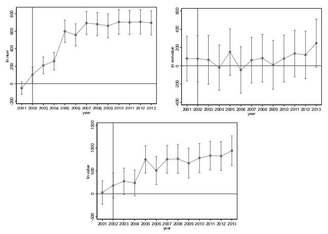
