1 Introduction
China now is the biggest carbon dioxide emitter in the world. Increased fossil-fuel consumption drove an estimated 2.3% increase in Chinese CO emissions in 2018, a second year of growth after emissions had appeared to level out between 2014 and 20161. The industry sector is highly energy-intensive, so the industry sector accounts for a large proportion of carbon dioxide emission2. Therefore, investigating the main factors that influence the carbon dioxide emission of the industry sector is of great importance.
1https://climateactiontracker.org/countries/china/.
2https://www.carbonbrief.org/guest-post-chinas-CO2-emissions-grew-slower-than-.
The iron and steel industry is the pillar industry of the industry sector and is the main source of energy consumption. China is the world's largest steel producer, manufacturing 716.5 million tons of crude steel in 2012, dwarfing the second-largest producer, Japan, which manufactures 107.2 million tons. While a few of China's large-scale mills are state-owned enterprises, most are small or medium scale and are privately run. Among the iron and steel, chemicals, and cement industries in China, the iron and steel industry emits the most greenhouse gases (2.015 GtCOe/year) and has the most abatement potential by 2030 (1.516 GtCOe/year). Greenhouse gas emissions within the iron and steel industry are linked directly to the traditional iron reduction process, which releases CO as a byproduct of iron ore and coking coal inputs3.
3https://sites.utexas.edu/mecc/2014/05/01/the-iron-and-steel-industry-in-china-part-i/.
According to China's Iron and Steel Association, the industry faces ongoing risks from excess capacity, as well as sluggish demand and increased raw material costs that could squeeze profits. Capacity cuts in 2016 progressed as planned by the Chinese government: A total of 65 million tons of iron and steel production capacity were closed, going beyond the annual target of 45 million tons. Also, this industry should work to avoid any illicit increase in new capacity, reduce leverage and push forward with the restructuring of "zombie firms"4.
4https://www.piie.com/blogs/china-economic-watch/chinas-excess-capacity-steel-fresh-look.
Although extensive research has examined the driving forces of China's iron and steel industry, few pieces of literature seek to find out the impact of capacity utilization on carbon dioxide emission in the iron and steel industry. What's more, numerous literature pays attention to industrial capacity utilization, but little has specially concentrated on industrial sub-sectors such as the iron and steel industry. Therefore, we carry out the empirical test by incorporating capacity utilization to the STIRPAT model as a core explanatory variable to explore the impact of capacity utilization on carbon dioxide emission in China's iron and steel industry and further dig the regional heterogeneity to find out more concrete findings.
When the government issues a series of de-capacity policies towards energy-consuming industries, raising capacity utilization is always mentioned as a policy target, so we use capacity utilization to measure the policy effect. By intensively reading the central and local government documents aimed at eliminating excess capacity, four channels can be summarized to raise the capacity utilization of China's iron and steel industry. First, by clearing below-standard capacity. Standards include environmental protection, consumption, safety quality, technology and so on. Clearing those backward capacity will reduce energy consumption and reduce carbon dioxide emission. Second, by encouraging iron and steel companies to conduct mergers and acquisitions so that several small-scale companies could become new large-scale companies through these two measures. Third, by guiding high-density capacity areas to transfer part of the existing capacity to other countries that are more environmentally appropriate to conduct steel production activities in order to release domestic capacity pressure. Pollution is also transferred during the process of transferring capacity, so carbon dioxide is also reduced. Last, by issuing a capacity replacement policy. It is required that new projects must eliminate equal or larger amounts of backward capacity, which leads to a more optimized capacity structure with less and less backward capacity. Through this method, overall backward capacity could be cleared indirectly, and carbon dioxide could be reduced.
Our main contributions are as follows: Firstly, we consider both excess capacity problem and environmental pollution problem, focus on a specific industrial sub-sector, the iron and steel industry, and find out the relationship between capacity utilization and carbon dioxide emission. Secondly, we explore regional heterogeneity and capacity-level heterogeneity to obtain more subtle and solid results. Thirdly, we expand the existing STIRPAT model by incorporating a new indicator (capacity utilization) and enrich the theory. Fourthly, we find out the mechanism of how capacity utilization influences carbon dioxide emission. Lastly, we novelly take energy consumption related variables as threshold variables to test different impacts of capacity utilization on carbon dioxide emission.
The rest of the paper is organized as follows: Section 2 briefly reviews the related and previous literature on CO emission in China's iron and steel industry and capacity utilization calculation. Section 3 describes the model specification, variable selection, and data description. Section 4 shows the empirical results of the benchmark model, mechanism analysis, robustness check, heterogeneity analysis from two perspectives, different regions, and different sub-samples and does some further analysis related to the topic. Section 5 summarizes the main findings of this paper and provides corresponding policy recommendations for policymakers.
2 Literature Review
1) Driving forces of carbon dioxide emission
China is currently the biggest carbon dioxide (CO
emitter in the world and the emission level differs in various regions in China. Low-carbon economy has become a heated topic and many scholars explore lowcarbon development pathways (Chen, et al.
[1], Wei, et al.
[2]). He, et al.
[3] examined the relationship between urbanization and CO
in China and divided 29 provinces into three regions according to economic development to further investigate the regional differences. As we mentioned China produces the largest amount of carbon dioxide and among the different industries the manufacturing industry is the biggest contributor to the emission and many scholars do extensive studies on industrial carbon emission (Xu, et al.
[4], Lin and Xu
[5], Karali, et al.
[6], Zhu, et al.
[7]). Xu, et al.
[4] showed that the CO
emission in the manufacturing industry accounted for more a half of the total emission of the whole of China and revealed the main driving forces of carbon dioxide emission in this industry using geographically weighted regression. Similarly this paper also divided the whole area into three regions, western, central and eastern regions, to investigate the regional difference. The results showed that in the manufacturing industry economic development has a positive impact on carbon dioxide emission in all three regions but the impact reduces from the eastern to the central and western. However, the impact of urbanization in the western region is higher than that in the eastern region and the central region. Lin and Xu
[5] also focused on the carbon dioxide emission of the manufacturing but different from most literature this paper divided the provinces into three categories according to the level of emission and applied the quantile regression approach to study the influencing factors of the carbon dioxide emission.
2) Conservation potential and carbon emission in iron and steel industry
An increasing number of scholars focus on the iron and steel industry and carry on a series of research on different aspects. The two main focuses are the conservation potential (Zhang, et al.
[8], An, et al.
[9], Wen, et al.
[10], Brunke and Blesl
[11], De Oliveira Junior, et al.
[12]), and carbon emission (Wang and Lin
[13], Tian, et al.
[14], Zhang, et al.
[15], Chen, et al.
[16], Hasanbeigi, et al.
[17], Peng, et al.
[18], Tang, et al.
[19]) of the iron and steel industry. The first branch of the literature mostly set different scenarios to predict the conservation potential of the iron and steel industry (An, et al.
[9], Wen, et al.
[10], Sheinbaum, et al.
[20]). Wen, et al.
[10] aimed to evaluate the potential for energy conservation of the iron and steel industry during 2010 and 2020 setting three scenarios including the business as usual scenario, the integrated policy scenario and the strengthened policy scenario based on the Asian-Pacific Integrated Model. Results showed that during the ten-year period technology promotion is the main driver for energy saving of the iron and steel industry. Zhang, et al.
[21] had the same outline of first setting a series of scenarios and then using these scenarios based on a specific model to predict the potential conservation ability of the iron and steel industry during a specific period. This paper sets four scenarios including the business-as-usual scenario, the structure adjustment scenario, the energy-efficiency improvement scenario, and the strengthened policy scenario based on the dynamic material flow analysis model to evaluate the conservation potential during 2015 and 2050.
3) Measuring of capacity utilization
Capacity utilization which is commonly defined as the ratio of actual capacity and potential capacity is another keyword of China's iron and steel industry. Current country-level policies such as the 12th five-year-plan, 13th five-year-plan and the supply-side reform all attach great importance to de-capacity especially in the energy-intensive and high-pollution industries including the iron and steel industry. Zhu, et al.
[22] presented a quantitative assessment of the emission trading scheme for China's iron and steel industry using simulation scenarios to find ways to help government effectively withdraw outdated capacity and better control the production of iron and steel industry and results showed that an output-based allocation approach is strongly recommended. The methods used to calculate the capacity utilization are divided into several categories and the most typical ones are data envelopment analysis (DEA), stochastic frontier analysis (SFA), production function analysis, cost function analysis and cointegration method. Yang and Fukuyama
[23] measured the capacity utilization of 30 provinces in China using a developed generalized capacity utilization indicator by modifying the data envelopment analysis model.
4) Summary of existing literature
Firstly, high energy consumption and overcapacity are two main features in China's iron and steel industry but few pieces of literature consider these two aspects in the same framework. So we explore the relationship of capacity utilization and carbon dioxide emission in China's iron and steel industry to link these two important aspects into one analysis framework. Secondly, most literature on capacity utilization is mainly studying the calculation of capacity utilization but few reveal the inner mechanism of how this will impact the carbon dioxide emission. In our paper, we introduce a mechanism of capacity utilization influencing carbon dioxide emission in the iron and steel industry with two main channels by our mechanism analysis.
3 Stylized Facts and Hypothesis
3.1 Stylized Facts
The iron and steel industry is the pillar industry of the industry sector and is the main source of energy consumption. China is the world's largest steel producer, manufacturing 716.5 million tons of crude steel in 2012, dwarfing the second-largest producer, Japan, which manufactures 107.2 million tons.
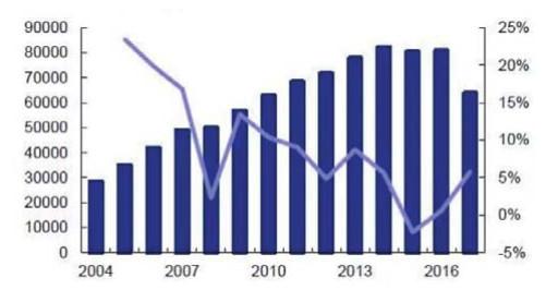
Figure 15 shows the trend of crude steel production information from 2004 to 2016. Crude steel is the most important product in the iron and steel industry, so the situation of crude steel output can, to some extent, reflect the situation of the iron and steel industry. Figure 1 shows that there is an upward trend from 2004 to 2014 in crude steel production of the whole country with a slight fall in 2014 to 2015 and remains the same in 2015 and 2016. In our research period, 2004–2015, crude steel production is progressively increasing gradually.
5 The graph is downloaded from https://www.sohu.com/a/210288440_99911594.
Figure 1 Crude steel output and growth rate of whole country from 2004 to 2016 |
Full size|PPT slide
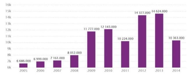
Figure 26 shows the trend of firm numbers of iron and steel industry from 2005 to 2014. It is generally showing an increasing trend except for two falls after 2010 and after 2013 respectively. The number of firms in the iron and steel industry is only 6686 in 2005, dramatically rising over 10000 in 2009 and reaches a peak in 2013.
6 The information is extracted from CEIC database.
Figure 2 Firm numbers from 2005–2014 in ISI |
Full size|PPT slide
3.2 Hypothesis
In this paper, we adopt capacity utilization to measure the de-capacity policies and introduce four primary hypotheses. Firstly, as we search and collect news and policies targeted toward the iron and steel industry, we find that most of these documents aim to raise capacity utilization and reduce carbon dioxide emissions. On the one hand, if capacity utilization is rising, the potential capacity will decline, which will possibly make the carbon dioxide emission decrease. On the other hand, when capacity utilization increases, the actual output of the iron and steel industry will increase, which may enlarge the scale of the industry and thus increase the carbon dioxide emission. Sun, et al.
[24] decomposed the driving factors of carbon dioxide emissions in the iron and steel industry in China and found that the production effect is the most important effect of increasing carbon emissions. Here we assume the latter is more realistic than the former one; therefore, the first hypothesis comes as:
H1 Capacity utilization and carbon dioxide emission in China's iron and steel industry are positively correlated.
Secondly, as China is a large country, different regions have different social and economic development level, and the capacity utilization of different regions also differ, which may lead to the different influence of capacity utilization and carbon dioxide emission in different areas. From the perspective of geographical location, most literature divides provinces into three regions, the eastern region, central region, and western region (Xu and Lin
[25], Chen, et al.
[26]). Different regions have different geographical features, different climate features, different economic development, different industrialization level, and different development targets. So some iron and steel firms may have the advantage to operate in a particular region while some may not. From the perspective of capacity utilization, it is necessary to see different results when considering different capacity utilization. It may be biased when ignoring the different levels of capacity utilization when testing the relationship between capacity utilization and carbon dioxide emission. So we assume that:
H2 The impact of capacity utilization on carbon dioxide emission in China's iron and steel industry differs in different regions divided by geographical location and level of capacity utilization.
Thirdly, by eliminating backward capacity and improving technology, the scale of the industry is enlarged, which will naturally bring about an increase in firm numbers, and thus there will be more energy consumption. When eliminating backward capacity, the output of the whole industry is increased. On the one hand, with the increase of output, mainly crude steel and pig iron, the scale of the industry is expanded. At the same time, international capacity cooperation is developing, which means more exporting firms are started. So firm number is increasing with the rising of actual output. When there are more firms in the industry, the production activities will be more active, which may lead to a rise in carbon dioxide emissions.
On the other hand, with the expansion of the iron and steel industry, there will be more energy consumption. The energy consumption trend is always consistent with the carbon dioxide emission (Sun, et al.
[27], Zhu, et al.
[7]), indicating that with more energy consumption in the iron and steel industry, the carbon dioxide emission may also increase. So our third hypothesis comes as:
H3 The impact of capacity utilization on carbon dioxide emission is influenced by the number of firms in the iron and steel industry and the total energy consumption.
Lastly, we already know the fact that carbon dioxide emission is closely related to energy consumption, so it is necessary to consider different levels of energy consumption when exploring the relationship between capacity utilization and carbon dioxide emission. With the energy consumption increasing, the relationship between those two may differ. Because energy consumption increasing also means a process of industrialization and urbanization, and different energy consumption levels indicate different development stages, which may make the de-capacity policies effectiveness differ. Since coal consumption is an essential kind of energy consumption, it is also vital to investigate whether there exist different impacts when the proportion of coal consumption changes. Because to some extent, energy structure also represents the level of usage of cleaner technology, which may influence the path of capacity utilization impacting carbon dioxide emissions. So here we assume that:
H4 The relationship between capacity utilization and carbon dioxide emission may vary in different levels of energy consumption and different proportion of coal consumption.
4 Model, Variable and Data
4.1 Benchmark Model and Variable Description
The STIRPAT model is often adopted to explore the driving forces of environmental pollution, especially carbon dioxide emission. Our paper aims to investigate the relationship between capacity utilization and carbon dioxide emission in China's iron and steel industry. Following previous literature such as (Lin and Xu
[5], Xu, et al.
[28], Xu and Lin
[29]) and (Xu and Lin
[30], Chen, et al.
[31]), we also apply the STIRPAT model to our paper and modify the original equation according to our topic. The pollution term can be substituted by CO
. Population size is the number of employees in the iron and steel industry, and technical progress is represented by the energy intensity of the industry. In order to seek the impact of capacity utilization on carbon dioxide emissions, we add an extra explanatory variable, capacity utilization, to the model. Capital stock and energy structure are also frequently used to measure the affluence level and technological progress level, so we incorporate these two factors into the equation to make the research more convincing. Considering the development and trade openness status of our country and on the purpose of digging the full influencing factors (Dong, et al.
[32]), we introduce industrialization, industrial structure, urbanization, and openness into the STIRPAT model as control variables. So the equation can be finally changed into the following form:
Equation (1) is the benchmark model of this paper. CO
represents CO
emissions from the IS industry in 28 provinces of China. It can be calculated from fossil fuel combustion through corresponding coefficients published by IPCC 2006.
represents capacity utilization which is defined as the ratio of actual output and potential output or the ratio of actual output and the data is extracted from (Deng et al.
[33]). The subscript
it in the variable indicates the
-th province in China in year
(2005–2014),
represents a random disturbance term. Control variables can be divided into two categories, one from the industry level and the other from the provincial level. First, the industry level control variables include 1) labor population (pop), representing the average number of employees in China's iron and steel industry; 2) energy structure (ens), representing the ratio of coal consumption of the iron and steel industry and the total energy consumption; 3) energy intensity (eni), calculated by dividing the total energy consumption by output; 4) capital stock (cap), calculated from the fixed assets investment in the IS industry. Second, the provincial level control variables include: 1) Economic level (gdp), representing per capita real GDP of each province, and has been converted into constant price; 2) Urbanization (urb), is the proportion of the urban population at the end of the year in the total population; 3) Industrialization (ind), is the ratio of the added value of the secondary industry and that of the whole industry; 4) The industrial structure (ins), representing the proportion of the added value of the secondary industry to that of the tertiary industry; 5) The trade openness (open), is calculated by dividing the sum of import and export by regional GDP.
4.2 Data
Carbon dioxide emission data can be calculated from fossil fuel combustion through corresponding coefficients published by IPCC 2006. Capacity utilization data is extracted from (Deng, et al.
[33]). All the other data is extracted from the China Statistical Yearbook (2006–2015), China Steel Statistical Yearbook (2006–2015), and the Provincial Statistical Yearbook (2006–2015). Due to a lack of data, three regions (Hainan Province, Chongqing, and Tibet Autonomous Region) are not included in the sample. The statistical description of all variables in our paper is shown in
Table 1.
Table 1 Data statistical description from 28 provinces in China from 2005 to 2014 |
| Variable | Definition | Unit | Mean | Std.Dev. | Min | Max |
| co2 | Carbon emission | Tce | 54795.4 | 53666.88 | 177.9852 | 295955 |
| pco2 | Per capita carbon emission | Tce | 4381.43 | 2586.73 | 37.34362 | 16694.8 |
| cu | Capacity utilization | % | 81.10832 | 3.808775 | 66.5543 | 90.0058 |
| ens | Energy structure | % | 4279.086 | 2021.627 | 9.505638 | 9121.873 |
| ener | Energy consumption | Tce | 2135.715 | 1858.994 | 173.5226 | 10814.7 |
| pop | Labor population | 104persons | 12.9632 | 11.45229 | 1.540001 | 62.16133 |
| cap | Capital stock | 108CNY | 426.6604 | 367.0158 | 21.44954 | 1809.979 |
| eni | Energy intensity | Tce/104CNY | 99114.43 | 54270.85 | 4500.664 | 371926.4 |
| firm | Number of firms | 1 | 288.6413 | 291.6926 | 19 | 1585 |
| gdp | Per capita real GDP | 104CNY/person | 15433.96 | 9624.245 | 2792.513 | 53237.93 |
| urb | Urbanization | % | 38.13746 | 17.0272 | 15.76 | 90.32 |
| ind | Industrialization | % | 48.37857 | 6.817611 | 21 | 59 |
| open | Trade openness | % | .3445978 | .4241041 | .03572 | 1.72148 |
| ins | Industrial structure | % | 126.015 | 31.19555 | 27.33921 | 205.4591 |
| Note: 1) all variables are converted into constant price. 2) Sample size is 280. |
4.3 Trend Analysis
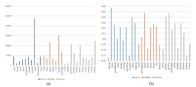
Figure 3(a) shows the carbon dioxide emission situation of each province and the carbon dioxide emission is the average of 2005–2014. From the general trend, the carbon dioxide emission is declined from eastern region to western region. Figure 3(b) demonstrates the capacity utilization of 10 year's average in each province, which shows a consistent trend with Figure 3(a).
Figure 3 Carbon emission and capacity utilization in ISI |
Full size|PPT slide
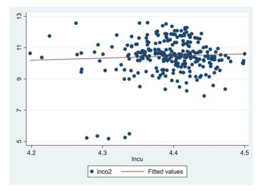
Figure 4 shows the scatter plot graph of capacity utilization and carbon dioxide emission in the iron and steel industry. Most scattered points are concentrated in the upper right of the coordinate system, so it can be preliminarily inferred that those two variables may be positively correlated. We further tested the non-linearity of the two variables, but the results showed that we should reject the non-linearity hypothesis7. So in this paper, we do not consider the non-linearity.
7We adopted the link test to investigate the non-linearity and the result showed that the non-linearity hypothesis should be rejected, which means the model should not incorporate higher order terms.
Figure 4 Scatter plot of capacity utilization and carbon dioxide emission in ISI |
Full size|PPT slide
5 Empirical Results and Discussion
In this section, we first analyze the general and basic impact of capacity utilization on carbon dioxide emission and then explore the mechanism of how capacity utilization influences carbon dioxide emission. After that, a robustness check is conducted to make the conclusion convincing. In addition, we consider heterogeneity to see the different impacts in different regions and different capacity utilization levels to get more subtle results. Finally, we further analyze the topic by adopting a panel threshold model to make our research more complete.
5.1 Benchmark Model Analysis
In this section, we aim to find out the basic impact of capacity utilization on carbon dioxide emission. The benchmark model result is shown in
Table 2. Fixed-effect (FE) method and Driscoll-Kray (DK) method are adopted. The fixed-effect model is widely used and can better eliminate the individual heterogeneous effects that cannot be observed over time, so it is more reasonable to use the FE method. Besides, the Hausman test also shows that the FE model is better than the random-effect model. DK methods provide standard errors for coefficients estimated by fixed-effect regression, and the size of the cross-sectional dimension in finite samples does not constitute a constraint on feasibility, so we also adopt this method to obtain our results (Chen, et al.
[31]).
Table 2 Regression results of benchmark model |
| | (a) | (b) | (c) | (d) | (e) | (f) |
| | DK0 | FE0 | DK1 | FE1 | DK | FE |
| ln cu | 0.229 | 0.229 | 1.099** | 1.099*** | 0.919** | 0.919** |
| | (0.917) | (0.857) | (0.526) | (0.361) | (0.445) | (0.355) |
| ln ens | | | 0.491*** | 0.491*** | 0.446*** | 0.446*** |
| | | | (0.0422) | (0.0258) | (0.0461) | (0.0259) |
| ln eni | | | 0.692*** | 0.692*** | 0.780*** | 0.780*** |
| | | | (0.0947) | (0.0613) | (0.0833) | (0.0620) |
| ln pop | | | 0.410*** | 0.410*** | 0.406*** | 0.406*** |
| | | | (0.0423) | (0.0684) | (0.0389) | (0.0659) |
| ln cap | | | 0.191** | 0.191*** | 0.120** | 0.120*** |
| | | | (0.0817) | (0.0403) | (0.0499) | (0.0432) |
| ln gdp | | | | | 0.155 | 0.155*** |
| | | | | | (0.0950) | (0.0593) |
| ln urb | | | | | 0.314*** | 0.314 |
| | | | | | (0.0853) | (0.193) |
| ln ind | | | | | 0.613** | 0.613 |
| | | | | | (0.224) | (0.634) |
| ln ins | | | | | 0.187 | 0.187 |
| | | | | | (0.112) | (0.324) |
| ln open | | | | | 0.0748 | 0.0748 |
| | | | | | (0.0654) | (0.0657) |
| Constant | 9.449** | 9.449** | 8.250** | 8.250*** | 11.52*** | 11.52*** |
| | (4.084) | (3.767) | (3.216) | (1.817) | (3.201) | (2.127) |
| Observations | 280 | 280 | 280 | 280 | 280 | 280 |
| -squared | | 0.000 | | 0.849 | | 0.869 |
| Number of groups | 28 | | 28 | | 28 | |
| Number of id | | 28 | | 28 | | 28 |
| Standard errors in parentheses, *** , ** , * . |
Column (a) contains only the core independent variable (capacity utilization) using DK regression. Column (b) changes to FE method. Column (c) and column (d) add four industrylevel control variables (energy structure, energy intensity, labor population and capital stock) using DK and FE respectively. Columns (e) and (f) incorporate all the control variables mentioned in Equation (6). Table 2 shows that before adding control variables, capacity utilization and carbon dioxide emission are positively related but the coefficients are not significant. After adding control variables, no matter adding only industrylevel control variables or adding both industrylevel and provinciallevel control variables, the coefficients are significantly positive and most control variables are significant. This result implies that the rise of capacity utilization will increase the carbon dioxide emission in China's iron and steel industry, which is consistent with Hypothesis 1 which holds the view that those two are positively correlated.
Intuitively, an increase in capacity utilization leads to a reduction in carbon emissions. However, the empirical evidence in this paper shows that an increase in capacity utilization will lead to a decrease in carbon emissions instead of an increase. Firstly, the media and academia have different measures of capacity utilization, with the media mostly choosing the ratio of supply to demand to measure capacity utilization. So because the media and academia have different definitions of capacity utilization, and we intuitively receive more influence from the media. The paper adopts the academic algorithm, resulting in opposite conclusions on the relationship between capacity utilization and carbon emissions intuitively and empirically. Secondly, our study interval is 2005–2014, with the policy of capacity removal increasing after 2016. However, before 2016, capacity removal policies were not effective enough, there was still a large amount of outdated capacity across the iron and steel industry, and production continued to increase. There is a real possibility that aggressive capacity policies could have increased carbon dioxide emissions instead of reducing them due to the lack of advanced clean technologies in the study interval.
5.2 Robustness Check
In this section, a robustness check is performed in various ways to make the result more convincing. Firstly, we substitute the dependent variable (carbon dioxide emission) into per capita carbon dioxide emission which is calculated by dividing the previous dependent variable by the population of the iron and steel industry. Secondly, we substitute the core independent variable (capacity utilization in log form) into the original form between 0 and 1. Thirdly, we change the calculation method of some control variables, urb which is the ratio of non-agricultural population and total population into urb2 which is the ratio of urban population and total population, gdp which is per capita real GDP into tgdp which represents the total real GDP. Except for capacity utilization, all the variables mentioned are in natural log form. Then, we try the random-effect model to test the robustness. Finally, we drop five observations with lnCO no bigger than 6 to see whether the result remains the same.
The robustness check result is shown in Table 3. Column (a) is the benchmark model regression. Column (b)(e) substitute dependent variable, core independent variable, control variable urb and control variable gdp. Column (f) is conducted under random-effect regression, and column (g) contains 275 observations. All the results are consistent with the benchmark model, which indicates that our results are robust, which again proves the Hypothesis 1 is correct.
Table 3 Results of robustness check |
| | (a) | (b) | (c) | (d) | (e) | (f) | (g) |
| VARIABLES | ln co2 | ln pco2 | ln co2 | ln co2 | ln co2 | ln co2 | ln co2 |
| ln cu | 0.919** | 0.917** | | 0.911** | 0.941*** | 0.942*** | 0.564** |
| | (0.355) | (0.355) | | (0.360) | (0.355) | (0.357) | (0.252) |
| cu_ori | | | 1.204*** | | | | |
| | | | (0.451) | | | | |
| ln ens | 0.446*** | 0.446*** | 0.446*** | 0.453*** | 0.448*** | 0.462*** | 0.132*** |
| | (0.0259) | (0.0259) | (0.0259) | (0.0267) | (0.0259) | (0.0252) | (0.0277) |
| ln eni | 0.780*** | 0.780*** | 0.780*** | 0.758*** | 0.783*** | 0.705*** | 0.432*** |
| | (0.0620) | (0.0620) | (0.0619) | (0.0636) | (0.0619) | (0.0587) | (0.0541) |
| ln pop | 0.406*** | 0.594*** | 0.408*** | 0.414*** | 0.409*** | 0.508*** | 0.146*** |
| | (0.0659) | (0.0658) | (0.0658) | (0.0668) | (0.0660) | (0.0579) | (0.0522) |
| ln cap | 0.120*** | 0.120*** | 0.121*** | 0.138*** | 0.121*** | 0.143*** | 0.0781** |
| | (0.0432) | (0.0432) | (0.0432) | (0.0439) | (0.0432) | (0.0418) | (0.0306) |
| ln gdp | 0.155*** | 0.155*** | 0.156*** | 0.244** | | 0.196*** | 0.416*** |
| | (0.0593) | (0.0593) | (0.0593) | (0.119) | | (0.0571) | (0.0454) |
| ln urb | 0.314 | 0.314 | 0.312 | | 0.306 | 0.389*** | 0.0636 |
| | (0.193) | (0.193) | (0.193) | | (0.192) | (0.150) | (0.137) |
| ln ind | 0.613 | 0.612 | 0.607 | 0.725 | 0.642 | 0.461 | 0.166 |
| | (0.634) | (0.634) | (0.634) | (0.635) | (0.631) | (0.604) | (0.450) |
| ln ins | 0.187 | 0.187 | 0.188 | 0.168 | 0.189 | 0.187 | 0.169 |
| | (0.324) | (0.324) | (0.324) | (0.325) | (0.325) | (0.309) | (0.230) |
| ln open | 0.0748 | 0.0747 | 0.0742 | 0.0905 | 0.0807 | 0.180*** | 0.0220 |
| | (0.0657) | (0.0657) | (0.0657) | (0.0694) | (0.0664) | (0.0520) | (0.0469) |
| ln urb2 | | | | 0.541 | | | |
| | | | | (0.431) | | | |
| ln tgdp | | | | | 0.142** | | |
| | | | | | (0.0552) | | |
| Constant | 11.52*** | 11.51*** | 8.455*** | 11.66*** | 11.58*** | 11.09*** | 3.812** |
| | (2.127) | (2.127) | (1.404) | (2.177) | (2.126) | (2.018) | (1.610) |
| Observations | 280 | 280 | 280 | 280 | 280 | 280 | 275 |
| -squared | 0.869 | 0.842 | 0.869 | 0.868 | 0.869 | 0.864 | 0.747 |
| Number of id | 28 | 28 | 28 | 28 | 28 | 28 | 28 |
5.3 Heterogeneity Analysis
In this section, we conduct the heterogeneity analysis from two perspective. Firstly, from regional perspective, the whole sample is divided into three regions, eastern, central and western regions. Secondly, from a sub-sample perspective, the whole sample is divided into three sub-samples according to different capacity utilization level.
5.3.1 Heterogeneity Analysis: Sub-Region
China is one of the largest countries in the world and has a large land area, which means that there may exist great regional heterogeneity among different areas. So it is necessary to divide the whole country area into some parts and examine the impact of capacity utilization on CO emission respectively to get more detailed and convincing information. In our paper, we follow most literature and the targeted 28 provinces are divided into three regions, the eastern region, central region, and western region. Table 4 shows the three regions in detail.
Table 4 Distribution of 28 administrative areas in the three regions of China |
| Region | Administrative areas (provinces, autonomous regions and municipalities) |
| eastern | Beijing, Tianjin, Hebei, Liaoning, Shanghai, Jiangsu, Zhejiang, Fujian, Shandong, Guangdong |
| central | Shanxi, Jilin, Heilongjiang, Anhui, Jiangxi, Henan, Hubei, Hunan |
| western | Inner Mongolia, Guangxi, Sichuan, Guizhou, Yunnan, Shaanxi, Gansu, Qinghai, Ningxia, Xinjiang |
Table 5 column (a)(d) shows the result of heterogeneity analysis considering regional differences. It can be seen that the coefficients of eastern and western regions are significantly positive which is in line with column (a), while the coefficient of the central region is not significant. When focusing on the absolute value of each region, it can be seen that the impact of capacity utilization on carbon dioxide emission in the western region is similar to that of the whole country which indicates that 1% raise of the capacity utilization in iron and steel industry will lead to about 0.9% increase of the carbon dioxide emission. This impact is smaller in the eastern region with an elasticity of about 0.5%. So, the impact of capacity utilization on carbon dioxide emission differs when considering the regional difference, which partly verifies Hypothesis 2.
Table 5 Results of heterogeneity analysis |
| | 1. Sub-region | | 2. Sub-sample-cu |
| (a) whole | (b) eastern | (c) central | (d) western | (e) Low-dk | (f) Low-fe | (g) Mid-dk | (h) Mid-fe | (i) High-dk | (j) High-fe |
| ln cu | 0.919** | 0.535** | 0.262 | 0.942** | | 0.478* | 0.478 | 1.725** | 1.725** | 0.646** | 0.646** |
| | (0.445) | (0.225) | (0.555) | (0.391) | (0.215) | (0.426) | (0.604) | (0.864) | (0.251) | (0.322) |
| ln ens | 0.446*** | 0.638*** | 0.0488** | 0.195*** | 0.327*** | 0.327*** | 0.513*** | 0.513*** | 0.0939*** | 0.0939*** |
| | (0.0461) | (0.0463) | (0.0182) | (0.0325) | (0.0789) | (0.0628) | (0.0230) | (0.0387) | (0.0258) | (0.0326) |
| ln eni | 0.780*** | 0.559*** | 0.255*** | 0.500*** | 0.345*** | 0.345*** | 0.833*** | 0.833*** | 0.373*** | 0.373*** |
| | (0.0833) | (0.108) | (0.0447) | (0.0678) | (0.0535) | (0.103) | (0.0766) | (0.100) | (0.0842) | (0.0763) |
| ln pop | 0.406*** | 0.135 | 0.375** | 0.217** | 0.129*** | 0.129 | 0.218*** | 0.218** | 0.277*** | 0.277*** |
| | (0.0389) | (0.0977) | (0.144) | (0.0690) | (0.0184) | (0.0936) | (0.0581) | (0.107) | (0.0379) | (0.0817) |
| ln cap | 0.120** | 0.0680 | 0.0399 | 0.138* | 0.375*** | 0.375*** | 0.0694 | 0.0694 | 0.109* | 0.109** |
| | (0.0499) | (0.132) | (0.0263) | (0.0646) | (0.0960) | (0.0767) | (0.0858) | (0.0694) | (0.0590) | (0.0449) |
| ln gdp | 0.155 | 0.270*** | 0.434*** | 0.419** | 0.318** | 0.318*** | 0.289 | 0.289* | 0.322*** | 0.322*** |
| | (0.0950) | (0.0815) | (0.0303) | (0.154) | (0.106) | (0.0813) | (0.169) | (0.149) | (0.0621) | (0.0760) |
| ln urb | 0.314*** | 0.928*** | 0.0363 | 0.313** | 0.610*** | 0.610*** | 0.426 | 0.426 | 0.552*** | 0.552 |
| | (0.0853) | (0.196) | (0.300) | (0.121) | (0.172) | (0.181) | (0.237) | (0.402) | (0.0982) | (0.351) |
| ln ind | 0.613** | 0.834 | 0.121 | 0.833 | 0.751** | 0.751 | 1.596*** | 1.596 | 0.414 | 0.414 |
| | (0.224) | (0.838) | (0.491) | (0.984) | (0.243) | (0.688) | (0.325) | (1.089) | (0.363) | (0.894) |
| ln ins | 0.187 | 0.208 | 0.288 | 0.759 | 0.713*** | 0.713** | 0.333 | 0.333 | 0.137 | 0.137 |
| | (0.112) | (0.508) | (0.267) | (0.487) | (0.135) | (0.343) | (0.211) | (0.554) | (0.134) | (0.426) |
| ln open | 0.0748 | 0.0921 | 0.179*** | 0.0308 | 0.0351 | 0.0351 | 0.199 | 0.199 | 0.0128 | 0.0128 |
| | (0.0654) | (0.191) | (0.0402) | (0.0537) | (0.0675) | (0.0983) | (0.152) | (0.170) | (0.0522) | (0.0570) |
| Constant | 11.52*** | 14.53*** | 0.408 | 5.751** | 2.885 | 2.885 | 18.17** | 18.17*** | 5.904** | 5.904** |
| | (3.201) | (3.319) | (3.343) | (1.852) | (1.743) | (2.933) | (5.598) | (4.841) | (2.579) | (2.454) |
| Observations | 280 | 100 | 80 | 100 | 90 | 90 | 90 | 90 | 100 | 100 |
| -squared | | | | | | 0.813 | | 0.954 | | 0.819 |
| Number of Groups | 28 | 10 | 8 | 10 | 9 | | 9 | | 10 | |
| Number of id | | | | | | 9 | | 9 | | 10 |
| Standard errors in parentheses, *** , ** , * . |
5.3.2 Heterogeneity Analysis: Sub-Sample
In this section, we divide the whole sample into three sub-samples according to different capacity utilization levels.
Table 5 columns (e) (g) (f) and columns (h) (i) (j) represent the low, middle, and high level of capacity utilization sub-sample regression results using DK and FE method respectively. The results of the DK and FE method are almost the same. Middle level and high level of capacity
5.4 Mechanism Analysis
In this section, we apply the mediation method to explore the mechanism of how capacity utilization impacts carbon dioxide emission. The iron and steel industry produces many different products. When observing the trend of the industry, the output of one or more main products can be a proper predictor. However, if using the output of one single product to be a mediation variable, the result will probably be biased. So two mediation variables are considered here, firm number (firm) and total energy consumption (ener). Mechanism 1 investigates how capacity utilization influences carbon dioxide emission through the change of firm numbers in the iron and steel industry. Mechanism 2 investigates how capacity utilization influences carbon dioxide emission through the change of total energy consumption in the iron and steel industry.
We first test Mechanism 1. When choosing firm number as the mediation variable, we can form three equations, Equation (2), Equation (3), and Equation (4), to investigate the mediation effect.
Table 6 shows the result of mechanism analysis using mediation tool. Columns (a)(c) represent the regression result of Equations (2)(4). The coefficient in Equation (2) is significantly positive, indicating the obvious positive relationship between capacity utilization and carbon dioxide emission. Among the coefficients in Equation (3) and in Equation (4) there is one significant and one insignificant, besides, the product of these two coefficients have the same sign with the coefficient in Equation (4), which means that firm number can be an effective mediation variable. The regression result also tells us that capacity utilization will first increase the number of firms in iron and steel industry and then the raise of the firm number will further increase the carbon dioxide emission.
Table 6 Results of mechanism analysis using mediation tool |
| | Mechanism 1 | | Mechanism 2 |
| (a) ln co2 | (b) ln firm | (c) ln co2 | (d) ln co2 | (e) ln ener | (f) ln co2 |
| ln cu | 0.919** | 0.0668 | 0.918** | | 0.919** | 0.828** | 0.440 |
| | (0.445) | (0.446) | (0.395) | (0.445) | (0.367) | (0.288) |
| ln firm | | | 0.0622** | | | |
| | | | (0.0242) | | | |
| ln ener | | | | | | 0.578*** |
| | | | | | | (0.0451) |
| ln ens | 0.446*** | 0.0638*** | 0.442*** | 0.446*** | 0.149*** | 0.533*** |
| | (0.0461) | (0.0109) | (0.0474) | (0.0461) | (0.0396) | (0.0345) |
| ln eni | 0.780*** | 0.00255 | 0.781*** | 0.780*** | 0.503*** | 0.489*** |
| | (0.0833) | (0.0401) | (0.0838) | (0.0833) | (0.130) | (0.0637) |
| ln pop | 0.406*** | 0.362*** | 0.383*** | 0.406*** | 0.309*** | 0.227*** |
| | (0.0389) | (0.0527) | (0.0412) | (0.0389) | (0.0806) | (0.0349) |
| ln cap | 0.120** | 0.0885*** | 0.127** | 0.120** | 0.228** | 0.0112 |
| | (0.0499) | (0.0199) | (0.0482) | (0.0499) | (0.106) | (0.0487) |
| ln gdp | 0.155 | 0.553*** | 0.119 | 0.155 | 0.00400 | 0.157* |
| | (0.0950) | (0.0358) | (0.0856) | (0.0950) | (0.0565) | (0.0769) |
| ln urb | 0.314*** | 0.578*** | 0.274*** | 0.314*** | 0.131* | 0.389*** |
| | (0.0853) | (0.0707) | (0.0760) | (0.0853) | (0.0763) | (0.0662) |
| ln ind | 0.613** | 0.223 | 0.596** | 0.613** | 1.007** | 0.0307 |
| | (0.224) | (0.308) | (0.231) | (0.224) | (0.377) | (0.361) |
| ln ins | 0.187 | 0.00690 | 0.186* | 0.187 | 0.0412 | 0.211 |
| | (0.112) | (0.209) | (0.109) | (0.112) | (0.185) | (0.159) |
| lnopen | 0.0748 | 0.0624 | 0.0706 | 0.0748 | 0.111 | 0.0106 |
| | (0.0654) | (0.0467) | (0.0696) | (0.0654) | (0.0884) | (0.0267) |
| Constant | 11.52*** | 0.229 | 11.52*** | 11.52*** | 7.193* | 7.359*** |
| | (3.201) | (2.042) | (2.968) | (3.201) | (3.852) | (1.887) |
| Observations | 280 | 276 | 276 | 280 | 280 | 280 |
| Number of groups | 28 | 28 | 28 | 28 | 28 | 28 |
| Standard errors in parentheses, *** , ** , * . |
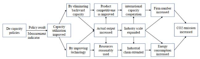
The inner logic can be revealed in Figure 5. A series of policies, no matter countrylevel policies or industrylevel policies, mainly aim to reduce existing capacity, possibly raising the ratio of actual output and potential output (that is to say, capacity). So raising capacity utilization can be the possible result of eliminating excess capacity and can be a measurement indicator to measure the effectiveness of the de-capacity policies. By eliminating backward capacity, the left capacity in the iron and steel industry is more effective and high-quality, so product competitiveness is raised and the output is increased. With the increase of output, mainly crude steel and pig iron, the scale of the industry is expanded. At the same time, international capacity cooperation is developing which means more exporting firms are started. So firm number is increasing with the rising of actual output. When there are more firms in the industry, the production activities will be more active which will, of course, lead to a rise in carbon dioxide emission. That is what Mechanism 1 indicates.
Figure 5 Mechanism of how capacity utilization influences CO2 emission |
Full size|PPT slide
We then test Mechanism 2 under a similar analyzing mode. When choosing total energy consumption as a mediation variable, we can form three equations, Equation (5), Equation (6), and Equation (7), to investigate the mediation effect.
Table 6 shows the result of mechanism analysis using a mediation tool. Columns (d)(f) represent the regression result of Equations (5)(7). The coefficient in Equation (5) is significantly positive, indicating the obvious positive relationship between capacity utilization and carbon dioxide emission. The coefficients in Equation (6) and in Equation (7) are both significant. Besides, the product of these two coefficients has the same sign with the coefficient in Equation (7), which means that energy consumption is a mediation variable. The regression result also tells us that capacity utilization will first increase energy consumption in the iron and steel industry and then due to more use of energy, the energy consumption will lead to more carbon dioxide emission.
The logit of how capacity influences carbon dioxide emission through energy consumption is also demonstrated in Figure 5. Capacity utilization can be raised by technical improvement aiming to reduce the use of blast furnaces in order to reduce existing capacity and increase capacity utilization. The technical improvement can make resources more reasonably allocated. At the same time, because of the increase of actual output and the scaling up of the industry, the iron and steel industry chain has been extended, reaching the construction industry, information industry, internet industry and so on. Naturally, the extension of the industry chain will possibly lead to more energy consumption which will further affect the emission of carbon dioxide.
5.5 Further Analysis: Panel Threshold Analysis
Panel threshold method is often used to capture different impacts when some specific variable reaches a specific value and this change will lead to different influences. Some literature studies the relationship of two variables considering the threshold effect (Hu, et al.
[34]). In their study, the relationship between the finance of land and the housing price at different stages of urbanization was studied.
From the previous sections above, we have known that there is a positive relationship between capacity utilization and carbon dioxide emission in China's iron and steel industry. In this section, in order to explore this relationship with more details, we conduct a panel threshold analysis to see whether there exists a threshold effect when using the proper variables. Both capacity utilization and carbon dioxide emission are closely related to energy using behavior. From the capacity utilization perspective, when adopting energy-friendly technology to improve the process of producing iron and steel, the capacity utilization would likely change. From the carbon dioxide emission perspective, both upstream and downstream iron and steel sub-industries will emit different amounts of carbon dioxide emission when energy consumption changes. Moreover, coal is the most used resource when consuming energy in the iron and steel industry, so the proportion of coal consumption to the total energy consumption, that is, energy structure, is also a vital factor that should not be ignored. So we first conduct panel threshold analysis using energy consumption as threshold variable and then further test the threshold effect using energy structure as threshold variable. Hopefully, we could offer more practical policy recommendations through analysis of this section.
In order to examine whether the impact of capacity utilization on carbon dioxide emission varies at different stages of energy consumption, the existence of an energy consumption threshold was tested firstly. As is shown in Table 7, value of the first threshold effect is 0.0000 and the null hypothesis that there is no threshold effect is rejected at a 1% significance level. The value of the double threshold effect is 0.0100, smaller than 0.05, indicating that the null hypothesis of no double threshold effect is rejected at a 5% significance level. The value of the triple threshold effect is 0.85, bigger than 0.1, failing to pass the significant test so the null hypothesis of no triple threshold effect is accepted. Therefore, it is inferred that energy consumption has a double threshold effect. The estimated thresholds are shown in Table 8 that the first threshold is 6.1709 and the second threshold is 6.4706.
Table 7 Results of threshold effect test — ener as threshold variable |
| | RSS | MSE | Fstat | Prob | Crit10 | Crit5 | Crit1 |
| Single | 6.9332 | 0.0257 | 70.97 | 0.0000 | 20.4414 | 23.7459 | 32.1148 |
| Double | 6.1587 | 0.0228 | 33.96 | 0.0100 | 20.1785 | 22.9699 | 33.6199 |
| Triple | 5.8272 | 0.0216 | 15.36 | 0.8500 | 56.9128 | 69.3663 | 88.1378 |
Table 8 Estimation of threshold value — ener as threshold variable |
| Threshold | Lower | Upper |
| 6.1709 | 6.1401 | 6.1743 |
| 6.4706 | 6.4682 | 6.5012 |
According to the two thresholds, the influence of capacity utilization on carbon dioxide emission can be divided into three energy using stages. As is shown in Table 9, the coefficients in the three stages are estimated as 0.6237479, 0.7189932, and 0.7832982 respectively, all passing the significance level of 5% which implies that at different stages of energy consumption, capacity utilization always influences carbon dioxide in a positive way. And the effect is gradually increasing in three stages, indicating that both thresholds are acceleration thresholds rather than deceleration thresholds. The positive impact of capacity utilization on carbon dioxide emission is gradually strengthening with more and more energy consumption used.
Table 9 Regression results of threshold effect — ener as threshold variable |
| variable | coefficient |
| ln pop | .3497018*** |
| ln eni | .6773857*** |
| ln ens | .4567278*** |
| ln cap | .0471033 |
| ln gdp | .1761238*** |
| ln urb | .3745906** |
| ln ind | .9210836* |
| ln ins ln open | .1377973.0544343 |
| ln enr | |
| ln ener | .6237479** |
| 6.1709ln ener | .7189932** |
| ln ener6.4706 | .7832982*** |
| cons | 8.812369*** |
| .9072 |
| 280 |
| Standard errors in parentheses, *** , ** , * . |
Similarly, we then test the threshold effect existence when using energy structure as the possible threshold variable. Table 10 shows that value of single threshold effect is 0.0000 which means that the null hypothesis of no threshold is rejected at 1% significance level. value of double threshold effect is 0.0833 indicating that the null hypothesis of no double threshold is rejected at 10% significance. But the hypothesis of that there existing no triple threshold effect should be accepted. So there are two thresholds and the estimated threshold value is shown in Table 11, 3.3095 and 8.6106 for the first the second threshold, respectively.
Table 10 Results of threshold effect test — ens as threshold variable |
| | RSS | MSE | Fstat | Prob | Crit10 | Crit5 | Crit1 |
| Single | 4.8544 | 0.0180 | 814.88 | 0.0000 | 20.5952 | 25.3858 | 33.7972 |
| Double | 4.5363 | 0.0168 | 18.94 | 0.0833 | 17.8898 | 24.5864 | 47.8467 |
| Triple | 4.2090 | 0.0156 | 20.99 | 0.3900 | 32.8838 | 36.6417 | 42.3223 |
Table 11 Estimation of threshold value — ens as threshold variable |
| Threshold | Lower | Upper |
| 3.3095 | 2.9992 | 4.2484 |
| 8.6106 | 8.5916 | 8.6215 |
According to the two thresholds, the influence of capacity utilization on carbon dioxide emission can be divided into three energy structure intervals. As is shown in Table 12, the coefficients in the three intervals are estimated as , 0.642364, and 0.6735227, respectively, with the first one failing to pass the significant test, the second one passing the 5% significant test and the third one passing the 1% significant test It implies that when there is a low proportion of coal consumption in total energy consumption, the capacity utilization and carbon dioxide emission is negatively correlated but not significant. As the proportion of coal consumption use expanding, the impact of capacity utilization on carbon dioxide turns positive and gradually increasing.
Table 12 Regression results of threshold effect — ens as threshold variable |
| variable | coefficient |
| ln pop | .1276792** |
| ln eni | .3487534*** |
| ln cap | .0612314** |
| ln gdp | .4575814*** |
| ln urb | .0122853 |
| ln ind | .536343 |
| ln ins | .0311117 |
| ln open | .0423495 |
| ln ens | |
| ln ens | .2615275 |
| ln ens | .642364** |
| ln ens | .6735227*** |
| cons | 3.114147* |
| .9320 |
| 280 |
| Standard errors in parentheses, *** , , * . |
6 Conclusion and Policy Recommendation
This paper explores the impact of capacity utilization on CO emissions in the industry, based on panel data of China's iron and steel (IS) industry from 2005 to 2014. The Benchmark model is used to test the basic positive relationship between capacity utilization and CO emissions in China's iron and steel industry. We also examine the heterogeneity of different regions in China and different levels of capacity utilization and carbon dioxide emission in sub-samples. What's more, two important mechanisms are found to support the positive impact of capacity utilization on carbon dioxide emission. Furthermore, at different thresholds of energy consumption and the ratio of coal consumption to total energy consumption, the impact differs. The main findings of this paper and policy recommendations are as follows.
The main conclusions are as follows. First, benchmark analysis shows that capacity utilization and carbon dioxide emission are positively related. This result implies that the rise of capacity utilization will increase the carbon dioxide emission in China's iron and steel industry. Second, when considering regional differences, it can be seen that the coefficients of eastern and western regions are significantly positive, which is in line with the benchmark result, while the coefficient of the central region is not significant. Therefore, the impact of capacity utilization on carbon dioxide emission differs when considering the regional difference. Third, two mechanisms are found as channels of capacity utilization impacting carbon dioxide emission. One channel is through the number of firms in the iron and steel industry. Capacity utilization will first increase the number of firms in the iron and steel industry, and then the rise of the firm number will further increase the carbon dioxide emission. The other channel is through energy consumption in the iron and steel industry. Capacity utilization will first increase energy consumption in the iron and steel industry, and then due to more use of energy, the energy consumption will lead to more carbon dioxide emission. Fourth, threshold effects are found to support the above findings further. At different stages of energy consumption, capacity utilization always positively influences carbon dioxide. The positive impact of capacity utilization on carbon dioxide emission is gradually strengthening with more energy consumption. When further considering the energy structure, different results come up. When there is a low proportion of coal consumption in total energy consumption, the capacity utilization, and carbon dioxide emission is negatively correlated but not significant. As the proportion of coal consumption uses expanding, the impact of capacity utilization on carbon dioxide turns positive and gradually increasing.
According to the findings of this paper and the current situation of the iron and steel industry, we put forward some policy recommendations for policymakers. First, as rising capacity utilization and reducing carbon dioxide emission have trade-offs, in order to achieve one of the positive policy effects, the government has to consider the negative effect brought out by the policy at the same time. Second, policies need to be tailored to the region and to other characteristics of the region (different capacity utilization levels or different carbon dioxide emission levels) in order to address the problems of the local iron and steel industry more efficiently. Third, establish an effective assessment system to include carbon emissions, overcapacity, capital, investment, and corresponding risks in the iron and steel industry as comprehensively as possible to make more accurate and comprehensive assessments and thus make more optimal decisions.
Despite the interesting findings of this paper, it also has some deficiencies. And we put forward some future research directions. First, the availability of data has to some extent, limited this paper. Future research could further enrich the current study if they could update the sample data to get the latest results. This paper covers data from the iron and steel industry at a provincial level, which could be extended to the city level in future studies. Second, more detailed research can be conducted on the mechanisms such as spatial measures or dynamic method. Besides, future research could evaluate the treatment effect of the policies in the iron and steel industry under the framework of counterfactual analysis. Third, we consider carbon dioxide emission into our analysis. Future research could add other environmental indicators such as solid dust, sulfur dioxide, PM2.5, and other air pollutants. Fourth, maybe international capacity cooperation could also be a possible mechanism in the path of capacity utilization impacting carbon dioxide emission and we will continue to explore possible mechanisms in future studies.
{{custom_sec.title}}
{{custom_sec.title}}
{{custom_sec.content}}
 PDF(356 KB)

 Figure 1 Crude steel output and growth rate of whole country from 2004 to 2016
 Table 1 Data statistical description from 28 provinces in China from 2005 to 2014


