A Vague Set Based OWA Method for Talent Evaluation

Peilong WANG; Dandan LI; Wei XU

doi:10.21078/JSSI-2023-0158

PDF(230 KB)

Journal of Systems Science and Information ›› 2024, Vol. 12 ›› Issue (4) : 543-553. DOI: 10.21078/JSSI-2023-0158

A Vague Set Based OWA Method for Talent Evaluation

Author information +

History +

Abstract

In recent years, decision-making under uncertainty has attracted substantial attention in both academia and industry, with a growing number of organizations prioritizing decision support for talent evaluation. Vague set theory has been recognized as a powerful tool to address the ambiguity of problem parameters and manage uncertainty. This paper introduces a novel talent evaluation method that harnesses the potential of vague sets. We construct a vague set Ordered Weighted Averaging (OWA) operator for offering a robust solution to intricate decision-making problems, especially in talent evaluation. The application of the OWA operator augments the decision-making process by providing a mechanism to handle the aggregation of information in a more flexible and comprehensive manner. Experimental results show the effectiveness of the proposed method, presenting an alternative for decision-makers, aiding them in selecting their preferred choices amidst uncertainty.

Key words

uncertain / vague set / talent evaluation / OWA operator

Cite this article

EndNote

Ris (Procite)

Bibtex

Download Citations

Peilong WANG , Dandan LI , Wei XU. A Vague Set Based OWA Method for Talent Evaluation. Journal of Systems Science and Information, 2024, 12(4): 543-553 https://doi.org/10.21078/JSSI-2023-0158

1 Introduction

Uncertain and noisy data, prevalent in economic, engineering, environmental, and social systems, pose challenges to conventional mathematical tools. However, they can be addressed using specialized theories and tools, such as fuzzy set theory^[1], rough set theory^[2], vague set theory^[3], intuitionistic fuzzy set theory^[4], and interval mathematics^{[5, 6]}. Each of these theories and tools has its unique advantages and inherent limitations^[7]. Recently, soft set theory, proposed by Molodtsov has been utilized to model problems characterized by complexity and uncertainty^[7]. A soft set is defined as a parameterized family of subsets of a universal set. Soft set theory has shown potential applications in various fields such as smoothness of functions, decision making, measurement theory, and game theory^[8].

Since 1999, soft set theory has received considerable attention in both theoretical and practical aspects. The basic concepts and properties of vague set theory have been formalized by Maji, et al.^[9], and new properties have been introduced^{[10, 11]}. In 2003, Maji, et al. developed fuzzy soft sets to fuzzy soft sets^[9]. Subsequently, specialized models including interval-valued fuzzy soft sets^[12], vague soft sets^[13], generalized fuzzy soft sets^{[14, 15]}, soft sets with description logics^[16], interval-valued intuitionistic fuzzy soft sets^[16], exclusive disjunctive soft sets^{[17, 18]}, and bijective soft sets^[19] have been developed as extensions to the soft sets. Soft sets have been integrated with related theories such as rough set theory, and algebra^{[20, 21]}. Moreover, soft set theory has been applied to feature selection^[22], forecasting^[23], clustering analysis^[24], and decision-making problems^[15-17].

Complex evaluation decision problems in uncertain environments pose significant challenges. Among the generalized set models, vague sets serve as an alternative tool for managing uncertainty, proving particularly useful in imprecise environments characterized by vagueness^[28]. This paper introduces a novel method for talent evaluation that harnesses the capabilities of vague sets. We construct an Ordered Weighted Averaging (OWA) operator using vague sets^[29]. This approach provides a robust solution to complex decision-making problems, especially in the realm of talent evaluation. The integration of the OWA operator enhances the decision-making process by offering a flexible and comprehensive mechanism for information aggregation.

The organization of this paper is as follows: Section 2 presents the fundamental definitions of vague sets and their properties. Section 3 illustrates an application of the proposed decision-making method in terms of vague sets to a complex decision-making problem. Finally, Section 4 provides conclusions and directions for future work.

2 Preliminaries

2.1 Vague Sets

In this section, the concepts of vague sets and their properties are summarized, whereas the details can be found in [28].

A vague set, denoted over a universe of discourse

U

U = {u_{1}, u_{2}, \dots, u_{n}}

, is distinguished by two membership functions: A truth-membership function, denoted as

t_{v}

, and a false-membership function

f_{v}

\begin{aligned} t_{v} : U \to [0, 1], \\ f_{v} : U \to [0, 1] . \end{aligned}

(1)

Here,

t_{v} (u_{i})

represents a lower bound on the grade of membership of

u_{i}

, which is derived from the evidence supporting

u_{i}

. Similarly,

f_{v} (u_{i})

is a lower bound on the negation of

u_{i}

, derived from the evidence against

u_{i}

, with the condition that

t_{v} (u_{i}) + f_{v} (u_{i}) \leq 1

. The grade of membership of

u_{i}

in the vague set is confined to a subinterval

[t_{v} (u_{i}), 1 - f_{v} (u_{i})]

of the interval

[0, 1]

. The vague value

[t_{v} (u_{i}), 1 - f_{v} (u_{i})]

suggests that the exact grade of membership

μ_{v} (u_{i})

u_{i}

might be unknown, but it is bounded by

t_{v} (u_{i}) \leq μ_{v} (u_{i}) \leq 1 - f_{v} (u_{i})

, where

t_{v} (u_{i}) + f_{v} (u_{i}) \leq 1

When the universe

U

is continuous, a vague set

A

can be expressed as

A = \int_{u_{i} \in U} [t_{A} (u_{i}), 1 - f_{A} (u_{i})] / u_{i},

(2)

where

u_{i} \in U

When the universe

U

is discrete, a vague set

A

can be expressed as

A = \sum_{i = 1}^{n} [t_{A} (u_{i}), 1 - f_{A} (u_{i})] / u_{i},

(3)

where $u_i \in U$.

For a vague set, [3] have introduced the following definitions concerning its operations, which will be useful to understand the subsequent discussion.

Definition 1 Let

x

be a vague value, denoted as

x = [t_{x}, 1 - f_{x}]

, where

t_{x} \in [0, 1]

f_{x} \in [0, 1]

, and

0 \leq t_{x} \leq 1 - f_{x} \leq 1

. If

t_{x} = 1

and

f_{x} = 0

(

i.e.,

x = [1, 1])

, then

x

is called a unit vague value. If

t_{x} = 0

and

f_{x} = 1

(i . e .,

x = [0, 0])

, then

x

is called a zero vague value.

Definition 2 Let

x

and

y

be two vague values, where

x = [t_{x}, 1 - f_{x}]

and

y = [t_{y}, 1 - f_{y}]

. If

t_{x} = t_{y}

and

f_{x} = f_{y}

, then vague values

x

and

y

are called equal

(i . e .,

[t_{x}, 1 - f_{x}] = [t_{y}, 1 - f_{y}])

For any two vague sets

X

and

Y

of the universe

U = {u_{1}, u_{2}, \dots, u_{n}}

, we have

\begin{aligned} X & = [t_{X} (u_{1}), 1 - f_{X} (u_{1})] / u_{1} + [t_{X} (u_{2}), 1 - f_{X} (u_{2})] / u_{2} + \dots + [t_{X} (u_{n}), 1 - f_{X} (u_{n})] / u_{n}, \\ Y & = [t_{Y} (u_{1}), 1 - f_{Y} (u_{1})] / u_{1} + [t_{Y} X (u_{2}), 1 - f_{Y} (u_{2})] / u_{2} + \dots + [t_{Y} (u_{n}), 1 - f_{Y} (u_{n})] / u_{n} . \end{aligned}

(4)

Definition 3 Let

X

be a vague set of the universe

U

. If

\forall u_{i} \in U

t_{X} (u_{1}) = 1

and

f_{A} (u_{i}) = 0

, then

X

is called a unit vague set, where

1 \leq i \leq n

. If

\forall u_{i} \in U

t_{X} (u_{i}) = 0

and

f_{A} (u_{i}) = 1

, then

X

is called a zero vague set,

1 \leq i \leq n

Definition 4 Let

X

be a vague set, the complement of

X

is denoted as

X^{c}

and defined as

\begin{aligned} t_{X}^{c} = F_{X}, \\ 1 - f_{X}^{c} = 1 - t_{X} . \end{aligned}

(5)

Definition 5 Assume that

A

and

B

are two vague sets of the universe

U

. Then the vague set

A

and

B

are equal if it satisfy

\forall u_{i} \in U

[t_{A} (u_{i}), 1 - f_{A} (u_{i})] = [t_{B} (u_{i}), 1 - f_{B} (u_{i}]

, where

1 \leq i \leq n

Definition 6 Assume that

A

and

B

are two vague sets of the universe

U

. The vague set

A

are included by

B

, denoted by

A \subseteq B

, if it satisfy

\forall u_{i} \in U

t_{A} (u_{i}) \leq t_{B} (u_{i})

and

1 - f_{A} (u_{i}) \leq 1 - f_{B} (u_{i})

, where

1 \leq i \leq n

Definition 7 Assume that

A

and

B

are two vague sets of the universe

U

C

is the union of them, i.e.,

C = A \cup B

, then the truth-membership and false-membership functions of

C

are defined as

\begin{aligned} t_{C} = max (t_{A}, t_{B}), \\ 1 - f_{C} = max (1 - f_{A}, 1 - f_{B}) = 1 - min (f_{A}, f_{B}) . \end{aligned}

(6)

Definition 8 Assume that

A

and

B

are two vague sets of the universe

U

C

is the intersection of them, i.e.,

C = A \cap B

, then the truth-membership and false-membership functions of

C

are defined as

\begin{aligned} t_{C} = min (t_{A}, t_{B}), \\ 1 - f_{C} = min (1 - f_{A}, 1 - f_{B}) = 1 - max (f_{A}, f_{B}) . \end{aligned}

(7)

2.2 Ordered Weighted Averaging Operator

Ordered Weighted Averaging, proposed by Yager^[30], essentially reorders data in descending order and assigns weights based on the position of the data before aggregating it.

Definition 9 Let

(α_{1}, α_{2}, \dots, α_{n})

be the decision vector with a related n-dimensional weight vector

ω = (ω_{1}, ω_{2}, \dots, ω_{n})

ω_{i} \in [0, 1], Σ_{i} ω_{i} = 1

. Then the OWA operator is

f_{O W A} : R^{n} \to R

, and given by

f_{O W A} (α_{1}, α_{2}, \dots, α_{n}) = \sum_{i = 1}^{n} ω_{i} b_{i}

(8)

where

b_{i}

is the jth value of

(α_{1}, α_{2}, \dots, α_{n})

in descending order.

OWA operator is wide used due to it's peculiarity to process data according to the desired attribute value type^[31]. The weight vector

ω

is associated with the OWA function. Administrators can set this according to practical circumstances and experience.

3 Methodology

In this section, we present an application of the proposed decision-making method, which utilizes vague sets to solve a complex evaluation problem. This is achieved with the assistance of multicriteria vague methods^{[32, 33]}. As an alternative to the comparison table proposed by Roy and Maji^[27], we develop a comparison score table and a weighted comparison score table to facilitate the decision-making process. The experimental results indicate that our proposed methods offer more valuable information than existing methods (e.g., Roy and Maji^[27]), thereby assisting decision-makers in making selections.

3.1 The Talent Evaluation Framework

As illustrated in Figure 1, we propose a comprehensive vague set-based OWA method to address the talent evaluation problem, aiming to assess the potential and performance of individuals across multiple criteria. The framework comprises five parts: Formulation of the decision support problem for talent evaluation, transformation into vague sets, score value calculation, application of the OWA operator for comprehensive attribute value, and talent ranking.

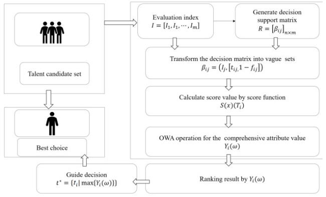
Figure 1 The framework of the proposed method

Full size|PPT slide

3.2 Linguistic Data Preparation

In the evaluation process, experts typically describe the candidate talent using the linguistic terms: 'Positive', 'Negative', and 'Abstention'. As per vague set theory, these linguistic evaluations can be converted into vague evaluations. For instance, for the candidate talent set

T = {T_{1}, T_{2}, \dots, T_{n}}

, there are

q

decision experts participating in the evaluation process.

Assume that the proportion of decision experts who consider the alternative

T_{i}

as 'Positive', 'Negative', and 'Abstention' are represented by

a_{i}

b_{i}

, and

c_{i}

for

i = 1, 2, \dots, n

, respectively. The vague evaluation of

T_{i}

is then denoted as

T_{i} = [t_{i}, 1 - f_{i}],

(9)

where

t_{i} = a_{i}

, and

f_{i} = b_{i}

for

i = 1, 2, \dots, n

. Here,

t_{i}

represents the degree to which decision experts are satisfied with

T_{i}

, and

f_{i}

represents the degree to which decision experts are not satisfied with

T_{i}

. Both

t_{i}

and

f_{i}

are in the interval

[0, 1]

, and the sum of

t_{i}

and

f_{i}

does not exceed 1, for all

i

such that

1 \leq i \leq m

. Specifically, a crisp value

x

, where

x \in [0, 1]

, can be represented by a vague value

[x, x]

. Next, we give an example to illustrate it.

Example 1 Assume that there is a group of decision experts with 10 members participating in the evaluation. If there are 5 participants who evaluate as 'Positive', 3 as 'Negative', and 2 as 'Abstention', then the proportions for the alternative are 0.5, 0.3, and 0.2, respectively. These proportions are denoted by

[0.5, 1 - 0.2]

3.3 The Talent Evaluation Problem

Consider the talent evaluation problem in the university recruitment process. Suppose the talent set is

T = {T_{1}, T_{2}, \dots, T_{n}}

, where

n

represents the number of candidates. The evaluation index set is

I = {I_{1}, I_{2}, \dots, I_{m}}

, where

m

represents the number of evaluation indexes. Each candidate

t_{i}

is measured according to the evaluation index set, but the attribute weight information is unknown. Assuming that the vague set

(t, 1 - f)

describes the academic achievement space, the problem is to identify an unknown talent from the vague data in terms of the vague set

(t, 1 - f)

. Thus, the decision scheme satisfies the degree of the evaluation index set

I = {I_{1}, I_{2}, \dots, I_{n}}

and can be represented by the decision matrix

R = (β_{i j})_{m \times n},

(10)

where

β_{i j} = (I_{j}, [t_{i j}, 1 - f_{i j}])

represents the degree to which the

i

-th decision scheme satisfies the

j

-th evaluation index. As discussed before, the evaluation index of candidate talent

T_{i}

are represented by the vague set as

T_{i} = {(I_{1}, [t_{i 1}, 1 - f_{i 1}]), (I_{2}, [t_{i 2}, 1 - f_{i 2}]), \dots, (I_{m}, [t_{i m}, 1 - f_{i m}])} .

(11)

In this context,

t_{i j}

denotes the extent to which the

i

-th candidate talent,

T_{i}

, fulfills the

j

-th evaluation index,

I_{j}

. Conversely,

f_{i j}

signifies the extent to which

T_{i}

fails to meet

I_{j}

. Both

t_{i j}

and

f_{i j}

are bounded by the interval

[0, 1]

, i.e.,

0 \leq t_{i j}, f_{i j} \leq 1

. Furthermore, the sum of

t_{i j}

and

f_{i j}

must not exceed 1, i.e.,

t_{i j} + f_{i j} \leq 1

. This holds true for all

i = 1, 2, \dots, n

and

j = 1, 2, \dots, m

. The characteristics of these candidate talents are summarized in Table 1.

Table 1 The tabular representation of the vague set

T	I₁	I₂	· · ·	I_m
T₁	[t₁₁, 1−f₁₁]	[t₁₂, 1−f₁₂]	· · ·	[t_1m, 1−f_1m]
T₂	[t₂₁, 1−f₂₁]	[t₂₂, 1−f₂₂]	· · ·	[t_2m, 1−f_2m]
⋮	⋮	⋮	⋱	⋮
T_n	[t_n1, 1−f_n1]	[t_n2, 1−f_n2]	· · ·	[t_nm, 1−f_nm]

3.4 Score Function for the Talent Evaluation Problem

In this subsection, the score function is introduced to solve the complex talent evaluation problem above. Let

x = [t_{x}, 1 - f_{x}]

be a vague value^[3], where

t_{x} \in [0, 1]

f_{x} \in [0, 1]

, and

t_{x} + f_{x} \leq 1

. The score of

x

can be evaluated by the score function

S

as:

S (x) = {\begin{aligned} 0, & f_{x} = t_{x} = 0, \\ \frac{t_{x} - f_{x}}{2} + \frac{t_{x} - f_{x}}{2 (t_{x} + f_{x})}, & others . \end{aligned}

(12)

As discussed in ^[34], the score function can get more consistent with people's intuitive judgement of the results of the reflection of the vague set of true-false affiliation of the absolute gap of the scoring function and reflect the relative gap of the scoring function of the two scoring function common characteristics. The table represent of evaluation score is shown in Table 2.

Table 2 The evaluation score value S(x) of all evaluation index set

T	I₁	I₂	T₃	· · ·	I_m
T₁	s₁₁	s₁₂	s₁₃	· · ·	s_1m
T₁	s₂₁	s₂₂	s₂₃	· · ·	s_2m
⋮	⋮	⋮	⋱	⋮
T_n	s_n1	s_n2	s_n3	· · ·	s_nm

3.5 OWA Operator for the Talent Evaluation

Considering the inherent complexity and diversity of talent evaluation systems, there is a high demand for sophisticated risk assessment methods. These methods must take into account unknown risks to ensure the maximization of talent selection for schools. This paper proposes a feasible evaluation system for decision-makers, assessing the current research level of talents based on the Ordered Weighted Averaging (OWA) operator. According to Definition, OWA operator is used to aggregate each risk factor

T_{i}

(i \in n)

, thus, get its comprehensive attribute value

Y_{i} (ω)

Y_{i} (ω) = O W A_{ω} (β_{i 1}, β_{i 2}, \dots, β_{i m}) = Σ_{j = 1}^{m} .

(13)

Then, based on the comprehensive attribute values obtained above, we perform a ranking for talent evaluation, determining the academic talent score based on scientific level. With the ranking score

{\tilde{T}}_{1} > {\tilde{T}}_{2} > \dots > {\tilde{T}}_{n}

where

Y_{1} (ω) > Y_{2} (ω) > \dots > Y_{n} (ω)

. Select the best talent by

T^{*} = {{\tilde{T}}_{1} | Y_{O W A} (T_{2}) = max {Y_{i} (ω), i = 1, 2, \dots, n}} .

(14)

3.6 The Process of the Talent Evaluation

In essence, the proposed method consists of five comprehensive steps, each of which plays a pivotal role in the overall evaluation process. The process is delineated as follows:

Step 1 The process begins with the generation of a decision matrix

R = (β_{i j})_{m \times n}

for the talent evaluation problem. This matrix encapsulates the evaluation scores of

n

talents across

m

criteria, thereby providing a structured approach to capture the multi-dimensional nature of talent evaluation.

Step 2 The decision matrix

R = (β_{i j})_{m \times n}

is then transformed into vague sets

β_{i j} = (I_{j}, [t_{i j}, 1 - f_{i j}])

. This transformation is integral to the methodology as it enables us to handle uncertainty and vagueness inherent in the evaluation scores, which are common phenomena in real-world talent evaluation scenarios.

Step 3 According to score function

S (x)

in Subsection 3.4 to measure the points under the criteria.

Step 4 Calculate the comprehensive attribute value

Y_{i} (ω)

according to OWA operator.

Step 5 Talent estimation and ranking according to

Y_{i} (ω)

, select the best talent

T_{i}

from them satisfy

max {Y_{i} (ω), i = 1, 2, \dots, n}

4 An Illustrate Example

This section takes an example to illustrate the proposed method. Let

T = {t_{1}, t_{2}, t_{3}, t_{4}, t_{5}, t_{6}}

denote the set of candidate talents. This study conducts talent evaluation based on four aspects: Teaching (Te), Scientific research (SR), Moral education (ME), and Social service (SS). The parameter set

I

encapsulates these four criteria, i.e.,

I = {Teaching, Scientific Research, Moral Education, Social Service} .

The detail calculate process are shown as below.

Step 1 In the process of evaluation, three linguistic terms, "Positive'', "Negative'', and "Abstention'' are provided for experts to evaluate the six candidate talents. Then the evaluation index sets are expressed as

I = {T e, S R, M E, S S}

. The number of experts who gave "Positive'', "Negative'', and "Abstention'' evaluations to the candidate talents under the four evaluation criteria is counted.

Step 2 Based on the approach proposed in Section 3, we transforme the linguistic evaluations of experts into vague sets as follows:

T_{1} = {(T e, [0.7, 0.8]), (S R, [0.8, 0.9]), (M E, [0.6, 0.8]), (S S, [0.8, 0.8])};

T_{2} = {(T e, [0.9, 0.9]), (S R, [0.8, 0.8]), (M E, [0.9, 1]), (S S, [0.8, 0.9])};

T_{3} = {(T e, [0.6, 0.7]), (S R, [0.7, 0.8]), (M E, [0.5, 0.6]), (S S, [0.9, 0.9])};

T_{4} = {(T e, [0.9, 0.9]), (S R, [0.6, 0.8]), (M E, [0.7, 0.8]), (S S, [0.7, 0.8])};

T_{5} = {(T e, [0.8, 0.9]), (S R, [0.9, 0.9]), (M E, [0.7, 0.7]), (S S, [0.8, 0.9])};

T_{6} = {(T e, [0.5, 0.6]), (S R, [0.7, 0.8]), (M E, [0.7, 0.9]), (S S, [0.9, 0.9])} .

Step 3 In the context of vague sets evaluation, this step computes the score values for all talents using the score function

S (x)

, as detailed in Subsection 3.4. The results are

T_{1}

S

(Te) = 0.475, S(SR) = 0.665,

S

(ME) = 0.360,

S

(SS) = 0.600;

T_{2}

S

(Te) = 0.800, S(SR) = 0.600,

S

(ME) = 0.855,

S

(SS) = 0.665;

T_{3}

S

(Te) = 0.475, S(SR) = 0.540,

S

(ME) = 0.095,

S

(SS) = 0.800;

T_{4}

S

(Te) = 0.800, S(SR) = 0.360,

S

(ME) = 0.540,

S

(SS) = 0.540;

T_{5}

S

(Te) = 0.665, S(SR) = 0.800,

S

(ME) = 0.600,

S

(SS) = 0.665;

T_{6}

S

(Te) = 0.360, S(SR) = 0.540,

S

(ME) = 0.400,

S

(SS) = 0.800.

Therefore, we can obtain the vague set evaluation decision score matrix as

\begin{matrix} T e S R M E S S \\ S (x) = \begin{matrix} T_{1} \\ T_{2} \\ T_{3} \\ T_{4} \\ T_{5} \\ T_{6} \end{matrix} (\begin{matrix} 0.475 & 0.665 & 0.360 & 0.600 \\ 0.800 & 0.600 & 0.360 & 0.600 \\ 0.475 & 0.540 & 0.095 & 0.665 \\ 0.800 & 0.360 & 0.540 & 0.540 \\ 0.665 & 0.800 & 0.600 & 0.665 \\ 0.360 & 0.540 & 0.400 & 0.800 \end{matrix}) . \end{matrix}

Step 4 Then we can obtain the sorted score value matrix of each talent

\begin{matrix} I_{1} I_{2} I_{3} I_{4} \\ \overset{⌢}{S} (x) = \begin{matrix} T_{1} \\ T_{2} \\ T_{3} \\ T_{4} \\ T_{5} \\ T_{6} \end{matrix} (\begin{matrix} 0.665 & 0.600 & 0.475 & 0.360 \\ 0.855 & 0.800 & 0.665 & 0.600 \\ 0.800 & 0.540 & 0.475 & 0.095 \\ 0.800 & 0.540 & 0.540 & 0.360 \\ 0.800 & 0.665 & 0.665 & 0.600 \\ 0.800 & 0.540 & 0.400 & 0.360 \end{matrix}) . \end{matrix}

Step 5 Calculate the comprehensive attribute

Y_{i} (ω)

using the OWA operator. The weight vector

ω = (0.287, 0.278, 0.230, 0.205)^{T}

is enacted based on past research and experience. Using Equation (), we can obtain the

Y_{O W A} (ω)

matrix

\begin{aligned} Y_{O W A} (ω) & = \hat{S} \times ω^{T} \\ = (\begin{array}{c} 0.665 & 0.600 & 0.475 & 0.360 \\ 0.855 & 0.800 & 0.665 & 0.600 \\ 0.800 & 0.540 & 0.475 & 0.095 \\ 0.800 & 0.540 & 0.540 & 0.360 \\ 0.800 & 0.665 & 0.665 & 0.600 \\ 0.800 & 0.540 & 0.400 & 0.360 \end{array}) \times (\begin{array}{c} 0.287 \\ 0.278 \\ 0.230 \\ 0.205 \end{array}) \\ = (\begin{array}{c} 0.665 * 0.287 + 0.600 * 0.278 + 0.475 * 0.230 + 0.360 * 0.205 \\ 0.855 * 0.287 + 0.800 * 0.278 + 0.665 * 0.230 + 0.600 * 0.205 \\ 0.800 * 0.287 + 0.540 * 0.278 + 0.475 * 0.230 + 0.095 * 0.205 \\ 0.800 * 0.287 + 0.540 * 0.278 + 0.540 * 0.230 + 0.360 * 0.205 \\ 0.800 * 0.287 + 0.665 * 0.278 + 0.665 * 0.230 + 0.600 * 0.205 \\ 0.800 * 0.287 + 0.540 * 0.278 + 0.400 * 0.230 + 0.360 * 0.205 \end{array}) = (\begin{array}{c} 0.5407 \\ 0.7437 \\ 0.5084 \\ 0.5777 \\ 0.6904 \\ 0.5455 \end{array}) . \end{aligned}

Therefore, we can be assembled value

Y_{i} (ω)

of the six talent

(T_{1}, T_{2}, T_{3}, T_{4}, T_{5}, T_{6})

as respectively: 0.5407, 0.7437, 0.5084, 0.5777, 0.6904, and 0.5455. This process allows us to quantitatively evaluate each talent and provides a basis for comparison and selection. The use of the OWA operator ensures that the evaluation is comprehensive, taking into account all available information about each talent.

Step 6 According to the results of numerical calculation, from big to small order available:

T_{2} ≻ T_{5} ≻ T_{4} ≻ T_{6} ≻ T_{1} ≻ T_{3},

and

Y_{O W A} (T_{2}) = max {Y_{i} (ω), i = 1, 2, \dots, 6} .

As a result,

T_{2}

can be assembled as the best candidate talent.

5 Discussions

In the discussion of the assembled values of the six talents

(T_{1}, T_{2}, T_{3}, T_{4}, T_{5}, T_{6})

, we have observed that the values are respectively: 0.5407, 0.7437, 0.5084, 0.5777, 0.6904, and 0.5455. This indicates a range of talent values with

T_{2}

having the highest value and

T_{3}

having the lowest. The numerical calculation results further support this observation by ranking the talents from highest to lowest as follows:

T_{2} ≻ T_{5} ≻ T_{4} ≻ T_{6} ≻ T_{1} ≻ T_{3}

. This ranking not only provides a clear hierarchy of the talents based on their assembled values but also highlights

T_{2}

as the talent with the maximum value among all. Therefore, based on both the assembled values and the results of numerical calculations, we can conclude that

T_{2}

is indeed the best talent among all. This conclusion provides valuable insights for decision-making processes where the selection of the best talent is crucial. However, it's also important to consider other factors such as context-specific requirements and constraints in real-world applications.

Overall, our methodology offers a systematic and rigorous approach to talent evaluation, effectively addressing its inherent challenges such as multi-dimensionality, uncertainty, and vagueness. It can be readily applied across various domains and adapted to meet specific needs.

6 Conclusions and Future Work

In this study, we introduce an innovative approach for talent assessment that utilizes the strengths of vague sets. We develop a vague set based OWA operator to provide a resilient solution to intricate decision-making challenges, specifically in the realm of talent evaluation. The incorporation of the OWA operator amplifies the decision-making procedure by offering a system to manage the consolidation of data in a more adaptable and exhaustive way. The empirical results validate the efficacy of the suggested method. It offers an alternative for decision-makers, assisting them in selecting their preferred choices amidst uncertainty. The proposed method is shown to provide more useful information than current methods in assisting decision makers to select choices. Further research can be done to measure the similarity of vague sets, and to study issues on the relationships among a vague set and other generalized sets. The proposed vague set based model can also be applied to solve other complex decision making problems with uncertainties.

References

Publishing order | Descend order by publishing year | Descend order by cited within

1	Zadeh L A. Fuzzy sets. Information and Control, 1965, 8, 338- 353. https://doi.org/10.1016/S0019-9958(65)90241-X Cited in this article [1]

2	Pawlak Z. Rough sets. International Journal of Information and Computer Sciences, 1982, 11, 341- 356. https://doi.org/10.1007/BF01001956 Cited in this article [1]

3	Gau W L, Buehrer D J. Vague sets. IEEE Transactions on Systems, Man and Cybernetics, 1993, 23 (2): 610- 614. https://doi.org/10.1109/21.229476 Cited in this article [3]

4	Atanassov K. Intuitionistic fuzzy sets. Fuzzy Sets and Systems, 1986, 20, 87- 96. https://doi.org/10.1016/S0165-0114(86)80034-3 Cited in this article [1]

5	Atanassov K. Operators over interval valued intuitionistic fuzzy sets. Fuzzy Sets and Systems, 1994, 64, 159- 174. https://doi.org/10.1016/0165-0114(94)90331-X Cited in this article [1]

6	Gorzalzany M B. A method of inference in approximate reasoning based on interval-valued fuzzy sets. Fuzzy Sets and Systems, 1987, 21, 1- 17. https://doi.org/10.1016/0165-0114(87)90148-5 Cited in this article [1]

7	Molodtsov D. Soft set theory - first results. Computers and Mathematics with Applications, 1999, 37 (4/5): 19- 31. Cited in this article [2]

8	Mohseni S, Pishvaee M S. Energy trading and scheduling in networked microgrids using fuzzy bargaining game theory and distributionally robust optimization. Applied Energy, 2023, 350, 121748. https://doi.org/10.1016/j.apenergy.2023.121748 Cited in this article [1]

9	Maji P K, Bismas R, Roy A R. Soft set theory. Computers and Mathematics with Applications, 2003, 45, 555- 562. https://doi.org/10.1016/S0898-1221(03)00016-6 Cited in this article [2]

10	Ali M I, Feng F, Liu X, et al. On some new operations in soft set theory. Computers and Mathematics with Applications, 2009, 57, 1547- 1553. https://doi.org/10.1016/j.camwa.2008.11.009 Cited in this article [1]

11	Yang C F. A note on "soft set theory". Computers and Mathematics with Applications, 2008, 56, 1899- 1900. https://doi.org/10.1016/j.camwa.2008.03.019 Cited in this article [1]

12	Yang X, Lin T Y, Yang J, et al. Combination of interval-valued fuzzy set and soft set. Computers and Mathematics with Applications, 2009, 58, 521- 527. https://doi.org/10.1016/j.camwa.2009.04.019 Cited in this article [1]

13	Sakr H H, Muse A H, Mohamed M S, et al. Applications on bipolar vague soft sets. Journal of Mathematics, 2023, 1- 25. Cited in this article [1]

14	Al-shami T M, Alcantud J C R, Mhemdi A. New generalization of fuzzy soft sets: $(a, b)$ -Fuzzy soft sets. AIMS Math, 2023, 8 (2): 2995- 3025. https://doi.org/10.3934/math.2023155 Cited in this article [1]

15	Majumdar P, Samanta S K. Generalised fuzzy soft sets. Computers and Mathematics with Applications, 2010, 59 (2): 787- 794. https://doi.org/10.1016/j.camwa.2009.10.015 Cited in this article [2]

16	Jiang Y, Tang Y, Chen Q, et al. Interval-valued intuitionistic fuzzy soft sets and their properties. Computers and Mathematics with Applications, 2010, 60, 906- 918. https://doi.org/10.1016/j.camwa.2010.05.036 Cited in this article [2]

17	Qasem M R, Salih M A, Noori S M. Soft set and its direct effect on a ring structure. Journal of Intelligent & Fuzzy Systems, 2020, 38 (3): 2885- 2888. Cited in this article [2]

18	Xiao Z, Gong K, Xia S, et al. Exclusive disjunctive soft sets. Computers and Mathematics with Applications, 2010. Cited in this article [1]

19	Gong K, Xiao Z, Zhang X. The bijective soft set with its operations. Computers and Mathematics with Applications, 2010, 60 (8): 2270- 2278. https://doi.org/10.1016/j.camwa.2010.08.017 Cited in this article [1]

20	Chen D, Tsang E C C, Yeung D S, et al. The parameterization reduction of soft sets and its applications. Computers and Mathematics with Applications, 2005, 49, 757- 763. https://doi.org/10.1016/j.camwa.2004.10.036 Cited in this article [1]

21	Tran D T, Huh J H. Building a model to exploit association rules and analyze purchasing behavior based on rough set theory. The Journal of Supercomputing, 2022, 78 (8): 11051- 11091. https://doi.org/10.1007/s11227-021-04275-5 Cited in this article [1]

22	Maharana M, Mohanty D. An application of soft set theory in decision making problem by parameterization reduction. Soft Computing, 2021, 25, 3989- 3992. https://doi.org/10.1007/s00500-020-05420-7 Cited in this article [1]

23	Xiao Z, Gong K, Zou Y. A combined forecasting approach based on fuzzy soft sets. Journal of Computational and Applied Mathematics, 2009, 228, 326- 333. https://doi.org/10.1016/j.cam.2008.09.033 Cited in this article [1]

24	Wang F. Aggregation similarity measure based on hesitant fuzzy closeness degree and its application to clustering analysis. Journal of Systems Science and Information, 2019, 7 (1): 70- 89. https://doi.org/10.21078/JSSI-2019-070-20 Cited in this article [1]

25	Jiang Y, Tang Y, Chen Q. An adjustable approach to intuitionistic fuzzy soft sets based decision making. Applied Mathematical Modelling, 2011, 35, 824- 836. https://doi.org/10.1016/j.apm.2010.07.038

26	Qian Y, Jun C, Ling T, et al. Hesitant trapezoid fuzzy hamacher aggregation operators and their application to multiple attribute decision making. Journal of Systems Science and Information, 2020, 8 (6): 524- 548. https://doi.org/10.21078/JSSI-2020-524-25

27	Roy A R, Maji P K. A fuzzy soft set theoretic approach to decision making problems. Journal of Computational and Applied Mathematics, 2007, 203, 412- 418. https://doi.org/10.1016/j.cam.2006.04.008 Cited in this article [2]

28	Xu W, Ma J, Wang S Y, et al. Vague soft sets and their properties. Computers and Mathematics with Applications, 2010, 59, 787- 794. https://doi.org/10.1016/j.camwa.2009.10.015 Cited in this article [2]

29	Luo C, Tian X, Wan S. Heavy OWA operator of trapezoidal intuitionistic fuzzy numbers and its application to multi-attribute decision making. Journal of Systems Science and Information, 2015, 3 (1): 86- 96. https://doi.org/10.1515/JSSI-2015-0086 Cited in this article [1]

30	Yager R R. On ordered weighted averaging aggregation operators in multi-criteria decision making. IEEE Transactions on Systems, Man and Cybernetics, 1988, 18 (1): 183- 190. https://doi.org/10.1109/21.87068 Cited in this article [1]

31	De Miguel L, Sesma-Sara M, Elkano M, et al. An algorithm for group decision making using $n$ -dimensional fuzzy sets, admissible orders and OWA operators. Computers & Mathematics with Applications, 2017, 74 (10): 2403- 2418. Cited in this article [1]

32	Chen S M, Tan J M. Handling multicriteria fuzzy decision-making problems based on vague set theory. Fuzzy Sets and Systems, 1994, 67, 163- 172. https://doi.org/10.1016/0165-0114(94)90084-1 Cited in this article [1]

33	Wang J, Liu S Y, Zhang J, et al. On the parameterized OWA operations for fuzzy MCDM based on vague set theory. Fuzzy Optimization and Decision Making, 2006, 5, 5- 20. https://doi.org/10.1007/s10700-005-4912-2 Cited in this article [1]

34	Zhang E Y, Wang J, Wang S Y. A new score function in multi-criteria decision making. System Science and Mathematics, 2011, 31 (8): 961- 974. Cited in this article [1]

Funding

the National Natural Science Foundation of China(72271233)

Suzhou Key Laboratory of Artificial Intelligence and Social Governance Technologies(SZS2023007)

Smart Social Governance Technology and Innovative Application Platform(YZCXPT2023101)

PDF(230 KB)

778

Accesses

Citation

Detail

Sections

Recommended

Received	Accepted
2023-10-15	2024-02-27
Issue Date
2024-08-16

Please choose a citation manager

Content to export

Abstract

Key words

Cite this article

1 Introduction

2 Preliminaries

2.1 Vague Sets

2.2 Ordered Weighted Averaging Operator

3 Methodology

3.1 The Talent Evaluation Framework

Figure 1 The framework of the proposed method

3.2 Linguistic Data Preparation

3.3 The Talent Evaluation Problem

Table 1 The tabular representation of the vague set

3.4 Score Function for the Talent Evaluation Problem

Table 2 The evaluation score value S(x) of all evaluation index set

3.5 OWA Operator for the Talent Evaluation

3.6 The Process of the Talent Evaluation

4 An Illustrate Example

5 Discussions

6 Conclusions and Future Work

{{custom_sec.title}}

{{custom_sec.title}}

References

{{custom_fnGroup.title_en}}

Footnotes

Funding

Share

模态框（Modal）标题

Please choose a citation manager

Content to export

Abstract

Key words

Cite this article

1 Introduction

2 Preliminaries

2.1 Vague Sets

2.2 Ordered Weighted Averaging Operator

3 Methodology

3.1 The Talent Evaluation Framework

Figure 1 The framework of the proposed method

3.2 Linguistic Data Preparation

3.3 The Talent Evaluation Problem

Table 1 The tabular representation of the vague set

3.4 Score Function for the Talent Evaluation Problem

Table 2 The evaluation score value S(x) of all evaluation index set

3.5 OWA Operator for the Talent Evaluation

3.6 The Process of the Talent Evaluation

4 An Illustrate Example

5 Discussions

6 Conclusions and Future Work

{{custom_sec.title}}

{{custom_sec.title}}

References

{{custom_fnGroup.title_en}}

Footnotes

Funding